Result Storage

This notebook will show how to store pypesto result objects to be able to load them later on for visualization and further analysis. This includes sampling, profiling and optimization. Additionally, we will show how to use optimization history to look further into an optimization run and how to store the history.

After this notebook, you will…

know how to store and load optimization, profiling and sampling results
know how to store and load optimization history
know basic plotting functions for optimization history to inspect optimization convergence

[1]:

# install if not done yet
# %pip install pypesto --quiet

Imports

[2]:

import logging
import random
import tempfile

import matplotlib as mpl
import matplotlib.pyplot as plt
import numpy as np
from IPython.display import Markdown, display

import pypesto.optimize as optimize
import pypesto.petab
import pypesto.profile as profile
import pypesto.sample as sample
import pypesto.visualize as visualize

mpl.rcParams["figure.dpi"] = 100
mpl.rcParams["font.size"] = 18
# set a random seed to get reproducible results
random.seed(3142)

%matplotlib inline

0. Objective function and problem definition

We will use the Boehm model from the benchmark initiative in this notebook as an example. We load the model through PEtab, a data format for specifying parameter estimation problems in systems biology.

[3]:

%%capture
# directory of the PEtab problem
petab_yaml = "./boehm_JProteomeRes2014/boehm_JProteomeRes2014.yaml"

importer = pypesto.petab.PetabImporter.from_yaml(petab_yaml)
problem = importer.create_problem(verbose=False)

1. Filling in the result file

We will now run a standard parameter estimation pipeline with this model. Aside from the part on the history, we shall not go into detail here, as this is covered in other tutorials such as Getting Started and AMICI in pyPESTO.

Optimization

[4]:

%%time

# create optimizers
optimizer = optimize.FidesOptimizer(
    verbose=logging.ERROR, options={"maxiter": 200}
)

# set number of starts
n_starts = 15  # usually a larger number >=100 is used

# Optimization
result = pypesto.optimize.minimize(
    problem=problem, optimizer=optimizer, n_starts=n_starts
)

2024-04-15 14:37:13.379 - amici.swig_wrappers - DEBUG - [model1_data1][CVODES:CVode:ERR_FAILURE] AMICI ERROR: in module CVODES in function CVode : At t = 145.387 and h = 3.81051e-05, the error test failed repeatedly or with |h| = hmin.

2024-04-15 14:37:13.380 - amici.swig_wrappers - ERROR - [model1_data1][FORWARD_FAILURE] AMICI forward simulation failed at t = 145.387: AMICI failed to integrate the forward problem

2024-04-15 14:37:15.556 - amici.swig_wrappers - DEBUG - [model1_data1][CVODES:CVode:ERR_FAILURE] AMICI ERROR: in module CVODES in function CVode : At t = 95.7183 and h = 1.99412e-05, the error test failed repeatedly or with |h| = hmin.

2024-04-15 14:37:15.557 - amici.swig_wrappers - ERROR - [model1_data1][FORWARD_FAILURE] AMICI forward simulation failed at t = 95.7183: AMICI failed to integrate the forward problem

2024-04-15 14:37:15.591 - amici.swig_wrappers - DEBUG - [model1_data1][CVODES:CVode:ERR_FAILURE] AMICI ERROR: in module CVODES in function CVode : At t = 95.4103 and h = 1.15865e-05, the error test failed repeatedly or with |h| = hmin.

2024-04-15 14:37:15.592 - amici.swig_wrappers - ERROR - [model1_data1][FORWARD_FAILURE] AMICI forward simulation failed at t = 95.4103: AMICI failed to integrate the forward problem

2024-04-15 14:37:15.684 - amici.swig_wrappers - DEBUG - [model1_data1][CVODES:CVode:ERR_FAILURE] AMICI ERROR: in module CVODES in function CVode : At t = 91.6716 and h = 1.10524e-05, the error test failed repeatedly or with |h| = hmin.

2024-04-15 14:37:15.685 - amici.swig_wrappers - ERROR - [model1_data1][FORWARD_FAILURE] AMICI forward simulation failed at t = 91.6716: AMICI failed to integrate the forward problem

2024-04-15 14:37:16.709 - amici.swig_wrappers - DEBUG - [model1_data1][CVODES:CVode:ERR_FAILURE] AMICI ERROR: in module CVODES in function CVode : At t = 146.181 and h = 3.10071e-06, the error test failed repeatedly or with |h| = hmin.

2024-04-15 14:37:16.710 - amici.swig_wrappers - ERROR - [model1_data1][FORWARD_FAILURE] AMICI forward simulation failed at t = 146.181: AMICI failed to integrate the forward problem

2024-04-15 14:37:16.928 - amici.swig_wrappers - DEBUG - [model1_data1][CVODES:CVode:ERR_FAILURE] AMICI ERROR: in module CVODES in function CVode : At t = 145.673 and h = 3.8101e-05, the error test failed repeatedly or with |h| = hmin.

2024-04-15 14:37:16.929 - amici.swig_wrappers - ERROR - [model1_data1][FORWARD_FAILURE] AMICI forward simulation failed at t = 145.673: AMICI failed to integrate the forward problem

2024-04-15 14:37:16.995 - amici.swig_wrappers - DEBUG - [model1_data1][CVODES:CVode:ERR_FAILURE] AMICI ERROR: in module CVODES in function CVode : At t = 145.587 and h = 1.77389e-05, the error test failed repeatedly or with |h| = hmin.

2024-04-15 14:37:16.996 - amici.swig_wrappers - ERROR - [model1_data1][FORWARD_FAILURE] AMICI forward simulation failed at t = 145.587: AMICI failed to integrate the forward problem

2024-04-15 14:37:17.044 - amici.swig_wrappers - DEBUG - [model1_data1][CVODES:CVode:ERR_FAILURE] AMICI ERROR: in module CVODES in function CVode : At t = 145.603 and h = 3.10559e-05, the error test failed repeatedly or with |h| = hmin.

2024-04-15 14:37:17.044 - amici.swig_wrappers - ERROR - [model1_data1][FORWARD_FAILURE] AMICI forward simulation failed at t = 145.603: AMICI failed to integrate the forward problem

2024-04-15 14:37:17.159 - amici.swig_wrappers - DEBUG - [model1_data1][CVODES:CVode:ERR_FAILURE] AMICI ERROR: in module CVODES in function CVode : At t = 89.1135 and h = 1.46515e-05, the error test failed repeatedly or with |h| = hmin.

2024-04-15 14:37:17.160 - amici.swig_wrappers - ERROR - [model1_data1][FORWARD_FAILURE] AMICI forward simulation failed at t = 89.1135: AMICI failed to integrate the forward problem

2024-04-15 14:37:20.823 - amici.swig_wrappers - DEBUG - [model1_data1][CVODES:CVode:ERR_FAILURE] AMICI ERROR: in module CVODES in function CVode : At t = 92.829 and h = 1.71535e-05, the error test failed repeatedly or with |h| = hmin.

2024-04-15 14:37:20.824 - amici.swig_wrappers - ERROR - [model1_data1][FORWARD_FAILURE] AMICI forward simulation failed at t = 92.829: AMICI failed to integrate the forward problem

2024-04-15 14:37:21.002 - amici.swig_wrappers - DEBUG - [model1_data1][CVODES:CVode:ERR_FAILURE] AMICI ERROR: in module CVODES in function CVode : At t = 89.3417 and h = 1.02033e-05, the error test failed repeatedly or with |h| = hmin.

2024-04-15 14:37:21.003 - amici.swig_wrappers - ERROR - [model1_data1][FORWARD_FAILURE] AMICI forward simulation failed at t = 89.3417: AMICI failed to integrate the forward problem

2024-04-15 14:37:21.214 - amici.swig_wrappers - DEBUG - [model1_data1][CVODES:CVode:ERR_FAILURE] AMICI ERROR: in module CVODES in function CVode : At t = 89.0734 and h = 1.56067e-05, the error test failed repeatedly or with |h| = hmin.

2024-04-15 14:37:21.214 - amici.swig_wrappers - ERROR - [model1_data1][FORWARD_FAILURE] AMICI forward simulation failed at t = 89.0734: AMICI failed to integrate the forward problem

2024-04-15 14:37:21.317 - amici.swig_wrappers - DEBUG - [model1_data1][CVODES:CVode:ERR_FAILURE] AMICI ERROR: in module CVODES in function CVode : At t = 145.721 and h = 3.00149e-05, the error test failed repeatedly or with |h| = hmin.

2024-04-15 14:37:21.317 - amici.swig_wrappers - ERROR - [model1_data1][FORWARD_FAILURE] AMICI forward simulation failed at t = 145.721: AMICI failed to integrate the forward problem

2024-04-15 14:37:21.944 - amici.swig_wrappers - DEBUG - [model1_data1][CVODES:CVode:ERR_FAILURE] AMICI ERROR: in module CVODES in function CVode : At t = 87.6456 and h = 1.21313e-05, the error test failed repeatedly or with |h| = hmin.

2024-04-15 14:37:21.944 - amici.swig_wrappers - ERROR - [model1_data1][FORWARD_FAILURE] AMICI forward simulation failed at t = 87.6456: AMICI failed to integrate the forward problem

2024-04-15 14:37:22.214 - amici.swig_wrappers - DEBUG - [model1_data1][CVODES:CVode:ERR_FAILURE] AMICI ERROR: in module CVODES in function CVode : At t = 145.564 and h = 2.81805e-05, the error test failed repeatedly or with |h| = hmin.

2024-04-15 14:37:22.215 - amici.swig_wrappers - ERROR - [model1_data1][FORWARD_FAILURE] AMICI forward simulation failed at t = 145.564: AMICI failed to integrate the forward problem

2024-04-15 14:37:24.361 - amici.swig_wrappers - DEBUG - [model1_data1][CVODES:CVode:ERR_FAILURE] AMICI ERROR: in module CVODES in function CVode : At t = 126.14 and h = 5.79296e-06, the error test failed repeatedly or with |h| = hmin.

2024-04-15 14:37:24.361 - amici.swig_wrappers - ERROR - [model1_data1][FORWARD_FAILURE] AMICI forward simulation failed at t = 126.14: AMICI failed to integrate the forward problem

2024-04-15 14:37:25.126 - amici.swig_wrappers - DEBUG - [model1_data1][CVODES:CVode:ERR_FAILURE] AMICI ERROR: in module CVODES in function CVode : At t = 145.607 and h = 3.21853e-06, the error test failed repeatedly or with |h| = hmin.

2024-04-15 14:37:25.127 - amici.swig_wrappers - ERROR - [model1_data1][FORWARD_FAILURE] AMICI forward simulation failed at t = 145.607: AMICI failed to integrate the forward problem

2024-04-15 14:37:25.211 - amici.swig_wrappers - DEBUG - [model1_data1][CVODES:CVode:ERR_FAILURE] AMICI ERROR: in module CVODES in function CVode : At t = 145.563 and h = 2.70563e-05, the error test failed repeatedly or with |h| = hmin.

2024-04-15 14:37:25.212 - amici.swig_wrappers - ERROR - [model1_data1][FORWARD_FAILURE] AMICI forward simulation failed at t = 145.563: AMICI failed to integrate the forward problem

CPU times: user 16.3 s, sys: 519 ms, total: 16.8 s
Wall time: 15.9 s

[5]:

display(Markdown(result.summary()))

Optimization Result

number of starts: 15
best value: 145.75946727842737, id=13
worst value: 249.7459981144093, id=3
number of non-finite values: 0
execution time summary:
- Mean execution time: 1.061s
- Maximum execution time: 2.034s, id=2
- Minimum execution time: 0.256s, id=3
summary of optimizer messages:

Count

Message

13

Converged according to fval difference

2

Trust Region Radius too small to proceed
best value found (approximately) 1 time(s)
number of plateaus found: 2

A summary of the best run:

Optimizer Result

optimizer used: <FidesOptimizer hessian_update=default verbose=40 options={‘maxiter’: 200}>
message: Converged according to fval difference
number of evaluations: 134
time taken to optimize: 1.654s
startpoint: [-2.36244359 1.67258019 -1.84421524 -4.05325559 -1.25299273 2.21184073 2.21608954 2.16674754 -1.62218154]
endpoint: [-1.5234124 -4.9981065 -2.03447661 -1.83084451 -1.67385748 3.941199 0.50778847 0.80382081 0.79608708]
final objective value: 145.75946727842737
final gradient value: [-0.0215125 0.02815549 -0.00217604 -0.02406847 -0.00935263 0.00867134 -0.00122642 0.0008237 0.00033701]
final hessian value: [[ 2.37341715e+03 3.60599720e-01 2.64777909e+02 2.61590175e+03 8.75220177e+02 -8.64898085e+02 6.91312132e+01 -4.51709055e+01 -2.39107733e+01] [ 3.60599720e-01 2.97611648e-04 2.95135049e-02 3.66326658e-01 1.61160365e-01 -1.71226537e-01 -1.69046982e-04 -2.71629785e-02 -3.74983901e-02] [ 2.64777909e+02 2.95135049e-02 7.03455663e+01 2.78309179e+02 1.49653353e+02 -1.35675484e+02 -3.38306768e+00 -3.46646434e-01 3.73472464e+00] [ 2.61590175e+03 3.66326658e-01 2.78309179e+02 2.91454367e+03 9.21987461e+02 -8.64616537e+02 8.16851512e+01 -4.77311580e+01 -3.38985735e+01] [ 8.75220177e+02 1.61160365e-01 1.49653353e+02 9.21987461e+02 4.25450232e+02 -4.03060118e+02 9.21380481e+00 -1.99689419e+01 1.07766723e+01] [-8.64898085e+02 -1.71226537e-01 -1.35675484e+02 -8.64616537e+02 -4.03060118e+02 1.14619635e+03 -2.12801326e+01 -1.23919635e+01 3.36521296e+01] [ 6.91312132e+01 -1.69046982e-04 -3.38306768e+00 8.16851512e+01 9.21380481e+00 -2.12801326e+01 8.48331937e+01 0.00000000e+00 0.00000000e+00] [-4.51709055e+01 -2.71629785e-02 -3.46646434e-01 -4.77311580e+01 -1.99689419e+01 -1.23919635e+01 0.00000000e+00 8.48284731e+01 0.00000000e+00] [-2.39107733e+01 -3.74983901e-02 3.73472464e+00 -3.38985735e+01 1.07766723e+01 3.36521296e+01 0.00000000e+00 0.00000000e+00 8.48295938e+01]]

Profiling

[6]:

%%time

# Profiling
result = profile.parameter_profile(
    problem=problem,
    result=result,
    optimizer=optimizer,
    profile_index=np.array([1, 1, 1, 0, 0, 0, 0, 0, 1]),
)

CPU times: user 5.54 s, sys: 292 ms, total: 5.83 s
Wall time: 5.37 s

Sampling

[7]:

%%time

# Sampling
sampler = sample.AdaptiveMetropolisSampler()
result = sample.sample(
    problem=problem,
    sampler=sampler,
    n_samples=5000,  # rather low
    result=result,
    filename=None,
)

Elapsed time: 15.990393325

CPU times: user 13.5 s, sys: 2.46 s, total: 16 s
Wall time: 12.4 s

2. Storing the result file

We filled all our analyses into one result file. We can now store this result object into HDF5 format to reload this later on.

[8]:

# create temporary file
fn = tempfile.NamedTemporaryFile(suffix=".hdf5", delete=False)
# write the result with the write_result function.
# Choose which parts of the result object to save with
# corresponding booleans.
pypesto.store.write_result(
    result=result,
    filename=fn.name,
    problem=True,
    optimize=True,
    profile=True,
    sample=True,
)

As easy as we can save the result object, we can also load it again:

[9]:

# load result with read_result function
result_loaded = pypesto.store.read_result(fn.name)

/home/docs/checkouts/readthedocs.org/user_builds/pypesto/envs/stable/lib/python3.11/site-packages/pypesto/store/read_from_hdf5.py:304: UserWarning: You are loading a problem. This problem is not to be used without a separately created objective.
  result.problem = pypesto_problem_reader.read()

As you can see, when loading the result object, we get a warning regarding the problem. This is the case, as the problem is not fully saved into hdf5, as a big part of the problem is the objective function. Therefore, after loading the result object, we cannot evaluate the objective function anymore. We can, however, still use the result object for plotting and further analysis.

The best practice would be to still create the problem through petab and insert it into the result object after loading it.

[10]:

# dummy call to non-existent objective function would fail
test_parameter = result.optimize_result[0].x[problem.x_free_indices]
# result_loaded.problem.objective(test_parameter)

[11]:

result_loaded.problem = problem
print(
    f"Objective function call: {result_loaded.problem.objective(test_parameter)}"
)
print(f"Corresponding saved value: {result_loaded.optimize_result[0].fval}")

Objective function call: 145.75946725797783
Corresponding saved value: 145.75946727842737

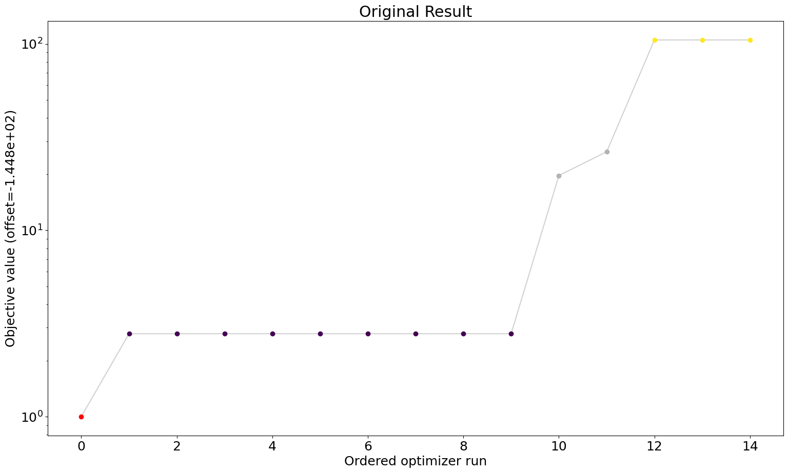
To show that for visualizations however, the storage and loading of the result object is accurate, we will plot some result visualizations.

3. Visualization Comparison

Optimization

[12]:

# waterfall plot original
ax = visualize.waterfall(result)
ax.title.set_text("Original Result")

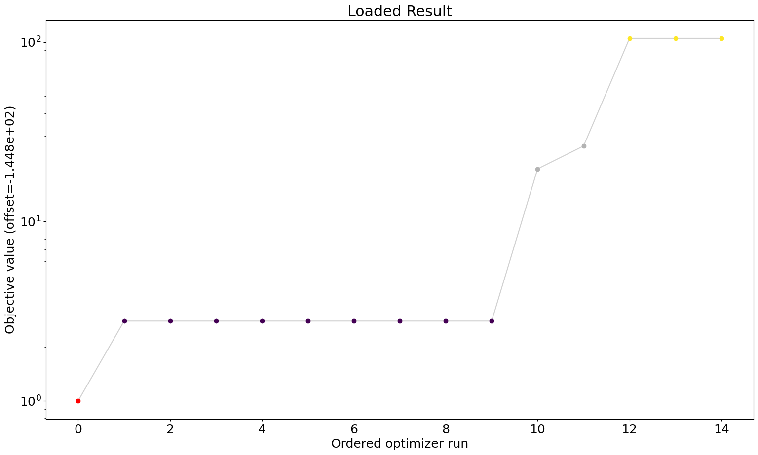
[13]:

# waterfall plot loaded
ax = visualize.waterfall(result_loaded)
ax.title.set_text("Loaded Result")

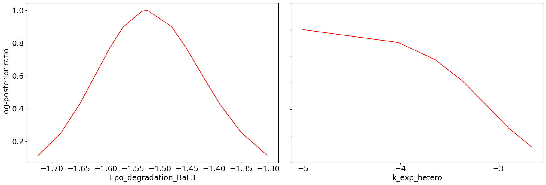
Profiling

[14]:

# profile plot original
ax = visualize.profiles(result)

[15]:

# profile plot loaded
ax = visualize.profiles(result_loaded)

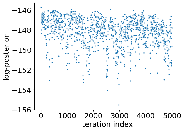
Sampling

[16]:

# sampling plot original
ax = visualize.sampling_fval_traces(result)

/home/docs/checkouts/readthedocs.org/user_builds/pypesto/envs/stable/lib/python3.11/site-packages/pypesto/visualize/sampling.py:79: UserWarning: Burn in index not found in the results, the full chain will be shown.
You may want to use, e.g., `pypesto.sample.geweke_test`.
  _, params_fval, _, _, _ = get_data_to_plot(

[17]:

# sampling plot loaded
ax = visualize.sampling_fval_traces(result_loaded)

/home/docs/checkouts/readthedocs.org/user_builds/pypesto/envs/stable/lib/python3.11/site-packages/pypesto/visualize/sampling.py:79: UserWarning: Burn in index not found in the results, the full chain will be shown.
You may want to use, e.g., `pypesto.sample.geweke_test`.
  _, params_fval, _, _, _ = get_data_to_plot(

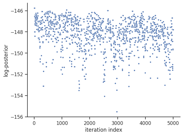
We can see that we are perfectly able to reproduce the plots from the loaded result object. With this, we can reuse the result object for further analysis and visualization again and again without spending time and resources on rerunning the analyses.

4. Optimization History

During optimization, it is possible to regularly write the objective function trace to file. This is useful, e.g., when runs fail, or for various diagnostics. Currently, pyPESTO can save histories to 3 backends: in-memory, as CSV files, or to HDF5 files.

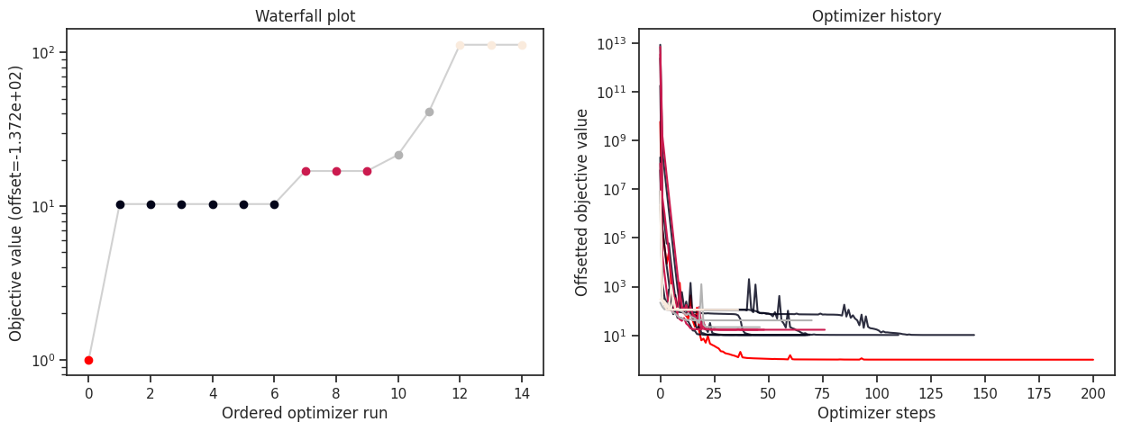
Memory History

To record the history in-memory, just set trace_record=True in the pypesto.HistoryOptions. Then, the optimization result contains those histories:

[18]:

# record the history
history_options = pypesto.HistoryOptions(trace_record=True)

# Run optimizations
result = optimize.minimize(
    problem=problem,
    optimizer=optimizer,
    n_starts=n_starts,
    history_options=history_options,
    filename=None,
)

2024-04-15 14:37:48.970 - amici.swig_wrappers - DEBUG - [model1_data1][CVODES:CVode:ERR_FAILURE] AMICI ERROR: in module CVODES in function CVode : At t = 129.941 and h = 5.48526e-06, the error test failed repeatedly or with |h| = hmin.

2024-04-15 14:37:48.971 - amici.swig_wrappers - ERROR - [model1_data1][FORWARD_FAILURE] AMICI forward simulation failed at t = 129.941: AMICI failed to integrate the forward problem

2024-04-15 14:37:51.234 - amici.swig_wrappers - DEBUG - [model1_data1][CVODES:CVode:ERR_FAILURE] AMICI ERROR: in module CVODES in function CVode : At t = 89.0261 and h = 1.13372e-05, the error test failed repeatedly or with |h| = hmin.

2024-04-15 14:37:51.234 - amici.swig_wrappers - ERROR - [model1_data1][FORWARD_FAILURE] AMICI forward simulation failed at t = 89.0261: AMICI failed to integrate the forward problem

2024-04-15 14:37:51.841 - amici.swig_wrappers - DEBUG - [model1_data1][CVODES:CVode:ERR_FAILURE] AMICI ERROR: in module CVODES in function CVode : At t = 88.0459 and h = 9.56593e-06, the error test failed repeatedly or with |h| = hmin.

2024-04-15 14:37:51.842 - amici.swig_wrappers - ERROR - [model1_data1][FORWARD_FAILURE] AMICI forward simulation failed at t = 88.0459: AMICI failed to integrate the forward problem

2024-04-15 14:37:52.046 - amici.swig_wrappers - DEBUG - [model1_data1][CVODES:CVode:ERR_FAILURE] AMICI ERROR: in module CVODES in function CVode : At t = 145.889 and h = 3.60065e-05, the error test failed repeatedly or with |h| = hmin.

2024-04-15 14:37:52.047 - amici.swig_wrappers - ERROR - [model1_data1][FORWARD_FAILURE] AMICI forward simulation failed at t = 145.889: AMICI failed to integrate the forward problem

2024-04-15 14:37:52.500 - amici.swig_wrappers - DEBUG - [model1_data1][CVODES:CVode:ERR_FAILURE] AMICI ERROR: in module CVODES in function CVode : At t = 89.0989 and h = 1.16981e-05, the error test failed repeatedly or with |h| = hmin.

2024-04-15 14:37:52.501 - amici.swig_wrappers - ERROR - [model1_data1][FORWARD_FAILURE] AMICI forward simulation failed at t = 89.0989: AMICI failed to integrate the forward problem

2024-04-15 14:37:53.437 - amici.swig_wrappers - DEBUG - [model1_data1][CVODES:CVode:ERR_FAILURE] AMICI ERROR: in module CVODES in function CVode : At t = 145.524 and h = 3.85325e-05, the error test failed repeatedly or with |h| = hmin.

2024-04-15 14:37:53.438 - amici.swig_wrappers - ERROR - [model1_data1][FORWARD_FAILURE] AMICI forward simulation failed at t = 145.524: AMICI failed to integrate the forward problem

2024-04-15 14:37:58.625 - amici.swig_wrappers - DEBUG - [model1_data1][CVODES:CVode:ERR_FAILURE] AMICI ERROR: in module CVODES in function CVode : At t = 146.52 and h = 3.55298e-05, the error test failed repeatedly or with |h| = hmin.

2024-04-15 14:37:58.626 - amici.swig_wrappers - ERROR - [model1_data1][FORWARD_FAILURE] AMICI forward simulation failed at t = 146.52: AMICI failed to integrate the forward problem

2024-04-15 14:37:58.906 - amici.swig_wrappers - DEBUG - [model1_data1][CVODES:CVode:ERR_FAILURE] AMICI ERROR: in module CVODES in function CVode : At t = 145.237 and h = 3.27774e-05, the error test failed repeatedly or with |h| = hmin.

2024-04-15 14:37:58.907 - amici.swig_wrappers - ERROR - [model1_data1][FORWARD_FAILURE] AMICI forward simulation failed at t = 145.237: AMICI failed to integrate the forward problem

2024-04-15 14:37:59.529 - amici.swig_wrappers - DEBUG - [model1_data1][CVODES:CVode:ERR_FAILURE] AMICI ERROR: in module CVODES in function CVode : At t = 10.1116 and h = 2.20871e-06, the error test failed repeatedly or with |h| = hmin.

2024-04-15 14:37:59.530 - amici.swig_wrappers - ERROR - [model1_data1][FORWARD_FAILURE] AMICI forward simulation failed at t = 10.1116: AMICI failed to integrate the forward problem

Now, in addition to queries on the result, we can also access the history.

[19]:

print("History type: ", type(result.optimize_result.list[0].history))
# print("Function value trace of best run: ", result.optimize_result.list[0].history.get_fval_trace())

fig, ax = plt.subplots(1, 2)
visualize.waterfall(result, ax=ax[0])
visualize.optimizer_history(result, ax=ax[1])
fig.set_size_inches((15, 5))

History type:  <class 'pypesto.history.memory.MemoryHistory'>

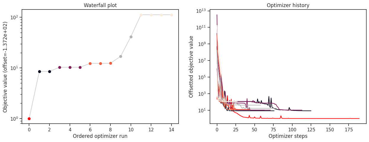
CSV History

The in-memory storage is, however, not stored anywhere. To do that, it is possible to store either to CSV or HDF5. This is specified via the storage_file option. If it ends in .csv, a pypesto.objective.history.CsvHistory will be employed; if it ends in .hdf5 a pypesto.objective.history.Hdf5History. Occurrences of the substring {id} in the filename are replaced by the multistart id, allowing to maintain a separate file per run (this is necessary for CSV as otherwise runs are overwritten).

[20]:

# create temporary file
with tempfile.NamedTemporaryFile(suffix="_{id}.csv") as fn_csv:
    # record the history and store to CSV
    history_options = pypesto.HistoryOptions(
        trace_record=True, storage_file=fn_csv.name
    )

    # Run optimizations
    result = optimize.minimize(
        problem=problem,
        optimizer=optimizer,
        n_starts=n_starts,
        history_options=history_options,
        filename=None,
    )

2024-04-15 14:38:28.825 - amici.swig_wrappers - DEBUG - [model1_data1][CVODES:CVode:ERR_FAILURE] AMICI ERROR: in module CVODES in function CVode : At t = 171.59 and h = 1.17045e-05, the error test failed repeatedly or with |h| = hmin.

2024-04-15 14:38:28.826 - amici.swig_wrappers - ERROR - [model1_data1][FORWARD_FAILURE] AMICI forward simulation failed at t = 171.59: AMICI failed to integrate the forward problem

2024-04-15 14:38:32.751 - amici.swig_wrappers - DEBUG - [model1_data1][CVODES:CVode:ERR_FAILURE] AMICI ERROR: in module CVODES in function CVode : At t = 72.2803 and h = 2.20177e-06, the error test failed repeatedly or with |h| = hmin.

2024-04-15 14:38:32.752 - amici.swig_wrappers - ERROR - [model1_data1][FORWARD_FAILURE] AMICI forward simulation failed at t = 72.2803: AMICI failed to integrate the forward problem

2024-04-15 14:38:32.809 - amici.swig_wrappers - DEBUG - [model1_data1][CVODES:CVode:ERR_FAILURE] AMICI ERROR: in module CVODES in function CVode : At t = 85.1756 and h = 9.29426e-06, the error test failed repeatedly or with |h| = hmin.

2024-04-15 14:38:32.810 - amici.swig_wrappers - ERROR - [model1_data1][FORWARD_FAILURE] AMICI forward simulation failed at t = 85.1756: AMICI failed to integrate the forward problem

2024-04-15 14:38:33.107 - amici.swig_wrappers - DEBUG - [model1_data1][CVODES:CVode:ERR_FAILURE] AMICI ERROR: in module CVODES in function CVode : At t = 88.1712 and h = 1.99775e-05, the error test failed repeatedly or with |h| = hmin.

2024-04-15 14:38:33.108 - amici.swig_wrappers - ERROR - [model1_data1][FORWARD_FAILURE] AMICI forward simulation failed at t = 88.1712: AMICI failed to integrate the forward problem

2024-04-15 14:38:33.254 - amici.swig_wrappers - DEBUG - [model1_data1][CVODES:CVode:ERR_FAILURE] AMICI ERROR: in module CVODES in function CVode : At t = 148.912 and h = 3.87866e-05, the error test failed repeatedly or with |h| = hmin.

2024-04-15 14:38:33.255 - amici.swig_wrappers - ERROR - [model1_data1][FORWARD_FAILURE] AMICI forward simulation failed at t = 148.912: AMICI failed to integrate the forward problem

Note that for this simple cost function, saving to CSV takes a considerable amount of time. This overhead decreases for more costly simulators, e.g., using ODE simulations via AMICI.

[21]:

print("History type: ", type(result.optimize_result.list[0].history))
# print("Function value trace of best run: ", result.optimize_result.list[0].history.get_fval_trace())

fig, ax = plt.subplots(1, 2)
visualize.waterfall(result, ax=ax[0])
visualize.optimizer_history(result, ax=ax[1])
fig.set_size_inches((15, 5))

History type:  <class 'pypesto.history.amici.CsvAmiciHistory'>

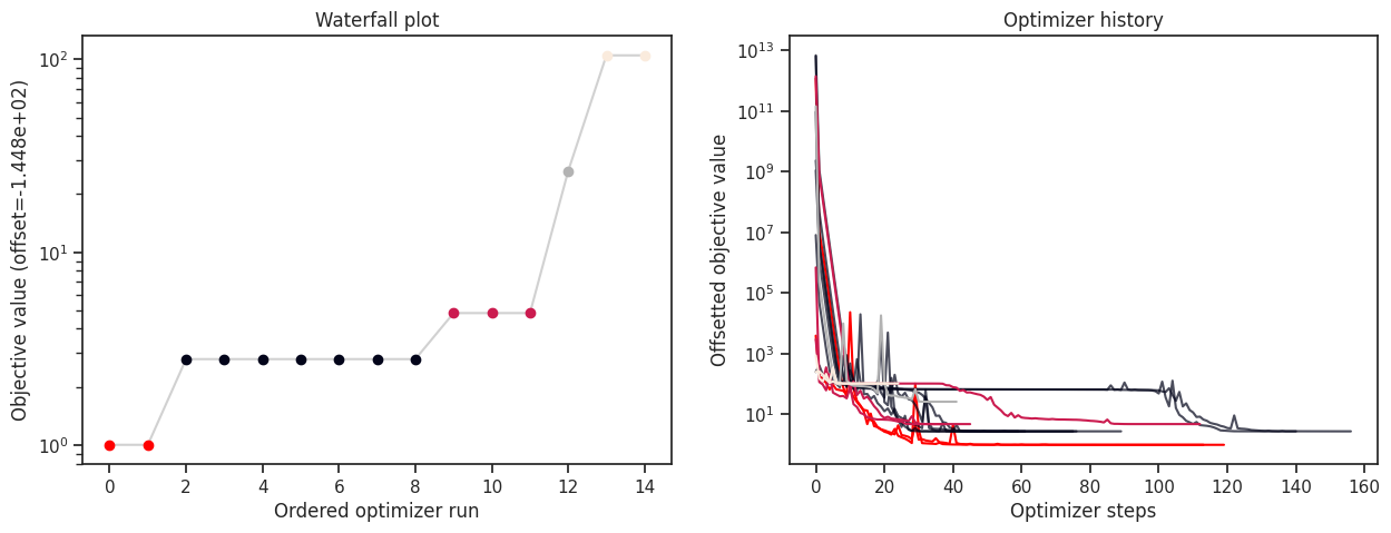
HDF5 History

Just as in CSV, writing the history to HDF5 takes a considerable amount of time. If a user specifies a HDF5 output file named my_results.hdf5 and uses a parallelization engine, then: * a folder is created to contain partial results, named my_results/ (the stem of the output filename) * files are created to store the results of each start, named my_results/my_results_{START_INDEX}.hdf5 * a file is created to store the combined result from all starts, named my_results.hdf5. Note that this file depends on the files in the my_results/ directory, so cease to function if my_results/ is deleted.

[22]:

# create temporary file
f_hdf5 = tempfile.NamedTemporaryFile(suffix=".hdf5", delete=False)
fn_hdf5 = f_hdf5.name

# record the history and store to CSV
history_options = pypesto.HistoryOptions(
    trace_record=True, storage_file=fn_hdf5
)

# Run optimizations
result = optimize.minimize(
    problem=problem,
    optimizer=optimizer,
    n_starts=n_starts,
    history_options=history_options,
    filename=fn_hdf5,
)

2024-04-15 14:38:36.779 - amici.swig_wrappers - DEBUG - [model1_data1][CVODES:CVode:ERR_FAILURE] AMICI ERROR: in module CVODES in function CVode : At t = 146.059 and h = 3.41214e-05, the error test failed repeatedly or with |h| = hmin.

2024-04-15 14:38:36.780 - amici.swig_wrappers - ERROR - [model1_data1][FORWARD_FAILURE] AMICI forward simulation failed at t = 146.059: AMICI failed to integrate the forward problem

2024-04-15 14:38:37.559 - amici.swig_wrappers - DEBUG - [model1_data1][CVODES:CVode:ERR_FAILURE] AMICI ERROR: in module CVODES in function CVode : At t = 101.504 and h = 2.39092e-06, the error test failed repeatedly or with |h| = hmin.

2024-04-15 14:38:37.560 - amici.swig_wrappers - ERROR - [model1_data1][FORWARD_FAILURE] AMICI forward simulation failed at t = 101.504: AMICI failed to integrate the forward problem

2024-04-15 14:38:38.219 - amici.swig_wrappers - DEBUG - [model1_data1][CVODES:CVode:ERR_FAILURE] AMICI ERROR: in module CVODES in function CVode : At t = 89.2149 and h = 1.43505e-05, the error test failed repeatedly or with |h| = hmin.

2024-04-15 14:38:38.220 - amici.swig_wrappers - ERROR - [model1_data1][FORWARD_FAILURE] AMICI forward simulation failed at t = 89.2149: AMICI failed to integrate the forward problem

2024-04-15 14:38:46.938 - amici.swig_wrappers - DEBUG - [model1_data1][CVODES:CVode:ERR_FAILURE] AMICI ERROR: in module CVODES in function CVode : At t = 89.0763 and h = 5.02801e-06, the error test failed repeatedly or with |h| = hmin.

2024-04-15 14:38:46.938 - amici.swig_wrappers - ERROR - [model1_data1][FORWARD_FAILURE] AMICI forward simulation failed at t = 89.0763: AMICI failed to integrate the forward problem

2024-04-15 14:38:47.108 - amici.swig_wrappers - DEBUG - [model1_data1][CVODES:CVode:ERR_FAILURE] AMICI ERROR: in module CVODES in function CVode : At t = 89.068 and h = 1.12459e-05, the error test failed repeatedly or with |h| = hmin.

2024-04-15 14:38:47.108 - amici.swig_wrappers - ERROR - [model1_data1][FORWARD_FAILURE] AMICI forward simulation failed at t = 89.068: AMICI failed to integrate the forward problem

2024-04-15 14:38:51.486 - amici.swig_wrappers - DEBUG - [model1_data1][CVODES:CVode:ERR_FAILURE] AMICI ERROR: in module CVODES in function CVode : At t = 62.4334 and h = 8.49555e-06, the error test failed repeatedly or with |h| = hmin.

2024-04-15 14:38:51.487 - amici.swig_wrappers - ERROR - [model1_data1][FORWARD_FAILURE] AMICI forward simulation failed at t = 62.4334: AMICI failed to integrate the forward problem

2024-04-15 14:38:51.654 - amici.swig_wrappers - DEBUG - [model1_data1][CVODES:CVode:ERR_FAILURE] AMICI ERROR: in module CVODES in function CVode : At t = 142.117 and h = 2.22987e-05, the error test failed repeatedly or with |h| = hmin.

2024-04-15 14:38:51.654 - amici.swig_wrappers - ERROR - [model1_data1][FORWARD_FAILURE] AMICI forward simulation failed at t = 142.117: AMICI failed to integrate the forward problem

2024-04-15 14:38:54.288 - amici.swig_wrappers - DEBUG - [model1_data1][CVODES:CVode:ERR_FAILURE] AMICI ERROR: in module CVODES in function CVode : At t = 155.231 and h = 3.51302e-05, the error test failed repeatedly or with |h| = hmin.

2024-04-15 14:38:54.288 - amici.swig_wrappers - ERROR - [model1_data1][FORWARD_FAILURE] AMICI forward simulation failed at t = 155.231: AMICI failed to integrate the forward problem

2024-04-15 14:38:57.290 - amici.swig_wrappers - DEBUG - [model1_data1][CVODES:CVode:ERR_FAILURE] AMICI ERROR: in module CVODES in function CVode : At t = 84.9791 and h = 2.32793e-06, the error test failed repeatedly or with |h| = hmin.

2024-04-15 14:38:57.291 - amici.swig_wrappers - ERROR - [model1_data1][FORWARD_FAILURE] AMICI forward simulation failed at t = 84.9791: AMICI failed to integrate the forward problem

2024-04-15 14:38:57.311 - amici.swig_wrappers - DEBUG - [model1_data1][CVODES:CVode:ERR_FAILURE] AMICI ERROR: in module CVODES in function CVode : At t = 80.9344 and h = 8.29933e-06, the error test failed repeatedly or with |h| = hmin.

2024-04-15 14:38:57.312 - amici.swig_wrappers - ERROR - [model1_data1][FORWARD_FAILURE] AMICI forward simulation failed at t = 80.9344: AMICI failed to integrate the forward problem

2024-04-15 14:38:57.581 - amici.swig_wrappers - DEBUG - [model1_data1][CVODES:CVode:ERR_FAILURE] AMICI ERROR: in module CVODES in function CVode : At t = 142.296 and h = 6.31185e-06, the error test failed repeatedly or with |h| = hmin.

2024-04-15 14:38:57.582 - amici.swig_wrappers - ERROR - [model1_data1][FORWARD_FAILURE] AMICI forward simulation failed at t = 142.296: AMICI failed to integrate the forward problem

[23]:

print("History type: ", type(result.optimize_result.list[0].history))
# print("Function value trace of best run: ", result.optimize_result.list[0].history.get_fval_trace())

fig, ax = plt.subplots(1, 2)
visualize.waterfall(result, ax=ax[0])
visualize.optimizer_history(result, ax=ax[1])
fig.set_size_inches((15, 5))

History type:  <class 'pypesto.history.amici.Hdf5AmiciHistory'>

For the HDF5 history, it is possible to load the history from file, and to plot it, together with the optimization result.

[24]:

# load the history
result_loaded_w_history = pypesto.store.read_result(fn_hdf5)

fig, ax = plt.subplots(1, 2)
visualize.waterfall(result_loaded_w_history, ax=ax[0])
visualize.optimizer_history(result_loaded_w_history, ax=ax[1])
fig.set_size_inches((15, 5))

/home/docs/checkouts/readthedocs.org/user_builds/pypesto/envs/stable/lib/python3.11/site-packages/pypesto/store/read_from_hdf5.py:304: UserWarning: You are loading a problem. This problem is not to be used without a separately created objective.
  result.problem = pypesto_problem_reader.read()

Loading the profiling result failed. It is highly likely that no profiling result exists within /tmp/tmp7_x90r02.hdf5.

Loading the sampling result failed. It is highly likely that no sampling result exists within /tmp/tmp7_x90r02.hdf5.

[25]:

# close the temporary file
f_hdf5.close()

Count	Message
13	Converged according to fval difference
2	Trust Region Radius too small to proceed