Prior definition

In this notebook we demonstrate how to include prior knowledge in a parameter inference problem, in particular how to define (log-)priors for parameters. If you want to maximize your posterior distribution, you need to define

• A (negative log-)likelihood

• A (log-)prior

The posterior is then built as an AggregatedObjective. If you import a problem via PEtab and the priors are contained in the parameter table, the definition of priors is done automatically.

CAUTION: The user needs to specify the negative log-likelihood, while the log-prior is internally multiplied by -1.

In this notebook:

• pypesto.objective.AggregatedObjective

• pypesto.objective.get_parameter_prior_dict

# install if not done yet
# %pip install pypesto --quiet

import numpy as np

import pypesto

Example: Rosenbrock Banana

We will use the Rosenbrock Banana

\begin{align} f(x, \theta) = \sum_{i=1}^{N} \underbrace{100 \cdot(x_{i}-x_{i-1}^2)^2}_{\text{"negative log-likelihood"}} + \underbrace{(x_{i-1}-1)^2}_{\text{"Gaussian log-prior"}} \end{align}

as an example. Here, we interpret the first term as the negative log-likelihood and the second term as Gaussian log-prior with mean \(1\) and standard deviation \(1/\sqrt{2}\).

Note that the second term is only equivalent to the negative log-distribution of a Gaussian up to a constant.

Define the negative log-likelihood

n_x = 5


def rosenbrock_part_1(x):
    """
    Calculate obj. fct + gradient of the "likelihood" part.
    """
    obj = sum(100.0 * (x[1:] - x[:-1] ** 2.0) ** 2.0)

    grad = np.zeros_like(x)
    grad[:-1] += -400 * (x[1:] - x[:-1] ** 2.0) * x[:-1]
    grad[1:] += 200 * (x[1:] - x[:-1] ** 2.0)

    return obj, grad


neg_log_likelihood = pypesto.Objective(fun=rosenbrock_part_1, grad=True)

Define the log-prior

A prior on an individual parameter is defined in a prior_dict, which contains the following key-value pairs:

• index: Index of the parameter

• density_fun: (Log-)posterior. (Scalar function!)

• density_dx: d/dx (Log-)posterior (optional)

• density_ddx: d^2/dx2 (Log-)posterior (optional)

A prior_dict can be either obtained by get_parameter_prior_dict for several common priors, or defined by the user.

from pypesto.objective.priors import get_parameter_prior_dict

# create a list of prior dicts...
prior_list = []
mean = 1
std_dev = 1 / np.sqrt(2)

for i in range(n_x - 1):
    prior_list.append(get_parameter_prior_dict(i, "normal", [mean, std_dev]))

# create the prior
neg_log_prior = pypesto.objective.NegLogParameterPriors(prior_list)

Define the negative log-posterior and the problem

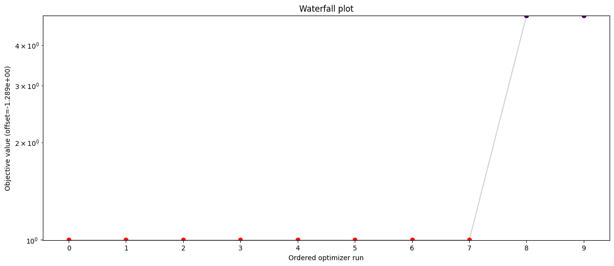
The negative log-posterior is defined as an AggregatedObjective. Since optimization/visualization is not the main focus of this notebook, the reader is referred to other examples for a more in-depth presentation of these. Here, basic visualisation is provided.

neg_log_posterior = pypesto.objective.AggregatedObjective(
    [neg_log_likelihood, neg_log_prior]
)

lb = -5 * np.ones((n_x, 1))
ub = 5 * np.ones((n_x, 1))

problem = pypesto.Problem(
    objective=neg_log_posterior,
    lb=lb,
    ub=ub,
)

Optimize

import pypesto.optimize as optimize

result = optimize.minimize(problem=problem, n_starts=10, filename=None)

Some basic visualizations

import pypesto.visualize as visualize

visualize.waterfall(result, size=(15, 6))

# parallel coordinates plot for best 5 fits
visualize.parameters(result, start_indices=5);