Hierarchical optimization with relative data
In this notebook we illustrate how to do hierarchical optimization in pyPESTO.
A frequent problem occuring in parameter estimation for dynamical systems is that the objective function takes a form
with data \(\bar y_i\), parameters \(\eta = (\theta,s,b,\sigma^2)\), and ODE simulations \(y(\theta)\). Here, we consider a Gaussian noise model, but also others (e.g. Laplace) are possible. Here we want to leverage that the parameter vector \(\eta\) can be split into “dynamic” parameters \(\theta\) that are required for simulating the ODE, and “static” parameters \(s,b,\sigma^2\) that are only required to scale the simulations and formulate the objective function. As simulating the ODE usually dominates the computational complexity, one can exploit this separation of parameters by formulating an outer optimization problem in which \(\theta\) is optimized, and an inner optimization problem in which \(s,b,\sigma^2\) are optimized conditioned on \(\theta\). This approach has shown to have superior performance to the classic approach of jointly optimizing \(\eta\).
In pyPESTO, we have implemented the algorithms developed in Loos et al.; Hierarchical optimization for the efficient parametrization of ODE models; Bioinformatics 2018 (covering Gaussian and Laplace noise models with gradients computed via forward sensitivity analysis) and Schmiester et al.; Efficient parameterization of large-scale dynamic models based on relative measurements; Bioinformatics 2019 (extending to offset parameters and adjoint sensitivity analysis).
However, the current implementation only supports:
Gaussian (normal) noise distributions
unbounded inner noise parameters \(\sigma\)
linearly-scaled inner parameters \(\eta\)
Scaling \(s\) and offset \(b\) parameters can be bounded arbitrarily.
In the following we will demonstrate how to use hierarchical optimization, and we will compare optimization results for the following scenarios:
Standard non-hierarchical gradient-based optimization with adjoint sensitivity analysis
Hierarchical gradient-based optimization with analytical inner solver and adjoint sensitivity analysis
Hierarchical gradient-based optimization with analytical inner solver and forward sensitivity analysis
Hierarchical gradient-based optimization with numerical inner solver and adjoint sensitivity analysis
[1]:
import time

import fides
import matplotlib.pyplot as plt
import numpy as np
from amici.sim.sundials import SensitivityMethod
from matplotlib.colors import to_rgba

import pypesto
from pypesto.hierarchical.relative import (
    AnalyticalInnerSolver,
    NumericalInnerSolver,
)
from pypesto.optimize.options import OptimizeOptions
from pypesto.petab import PetabImporter
Note on inclusion of additional data types:
It is possible to include observables with different types of data to the same petab_problem. Refer to the notebooks on using semiquantitative data, ordinal data and censored data for details on integration of other data types.
Problem specification
We consider a version of the [Boehm et al.; Journal of Proeome Research 2014] model, modified to include scalings \(s\), offsets \(b\), and noise parameters \(\sigma^2\).
NB: We load two PEtab problems here, because the employed standard and hierarchical optimization methods have different expectations for parameter bounds. The difference between the two PEtab problems is that the corrected_bounds version estimates inner noise parameters (\(\sigma\)) in \([0, \infty]\).
[2]:
# get the PEtab problem
# requires installation of
from pypesto.testing.examples import (
    get_Boehm_JProteomeRes2014_hierarchical_petab,
    get_Boehm_JProteomeRes2014_hierarchical_petab_corrected_bounds,
)

petab_problem = get_Boehm_JProteomeRes2014_hierarchical_petab()
petab_problem_hierarchical = (
    get_Boehm_JProteomeRes2014_hierarchical_petab_corrected_bounds()
)
To convert a non-hierarchical PEtab model to a hierarchical one, the observable_df, the measurement_df and the parameter_df have to be changed accordingly. The PEtab observable table contains placeholders for scaling parameters \(s\) (observableParameter1_{pSTAT5A_rel,pSTAT5B_rel,rSTAT5A_rel}), offsets \(b\) (observableParameter2_{pSTAT5A_rel,pSTAT5B_rel,rSTAT5A_rel}), and noise parameters \(\sigma^2\) (noiseParameter1_{pSTAT5A_rel,pSTAT5B_rel,rSTAT5A_rel}) that are
overridden by the {observable,noise}Parameters column in the measurement table.
N.B.: in general, the inner parameters can appear in observable formulae directly. For example, the first observable formula in this table could be changed from observableParameter2_pSTAT5A_rel + observableParameter1_pSTAT5A_rel * (100 * pApB + 200 * pApA * specC17) / (pApB + STAT5A * specC17 + 2 * pApA * specC17) to offset_pSTAT5A_rel + scaling_pSTAT5A_rel * (100 * pApB + 200 * pApA * specC17) / (pApB + STAT5A * specC17 + 2 * pApA * specC17).
Observable DF:
[3]:
from pandas import option_context

with option_context("display.max_colwidth", 400):
    display(petab_problem_hierarchical.observable_df)
| observableName | observableFormula | noiseFormula | observableTransformation | noiseDistribution | |
|---|---|---|---|---|---|
| observableId | |||||
| pSTAT5A_rel | NaN | observableParameter2_pSTAT5A_rel + observableParameter1_pSTAT5A_rel * (100 * pApB + 200 * pApA * specC17) / (pApB + STAT5A * specC17 + 2 * pApA * specC17) | noiseParameter1_pSTAT5A_rel | lin | normal |
| pSTAT5B_rel | NaN | observableParameter2_pSTAT5B_rel + observableParameter1_pSTAT5B_rel * -(100 * pApB - 200 * pBpB * (specC17 - 1)) / ((STAT5B * (specC17 - 1) - pApB) + 2 * pBpB * (specC17 - 1)) | noiseParameter1_pSTAT5B_rel | lin | normal |
| rSTAT5A_rel | NaN | observableParameter2_rSTAT5A_rel + observableParameter1_rSTAT5A_rel * (100 * pApB + 100 * STAT5A * specC17 + 200 * pApA * specC17) / (2 * pApB + STAT5A * specC17 + 2 * pApA * specC17 - STAT5B * (specC17 - 1) - 2 * pBpB * (specC17 - 1)) | noiseParameter1_rSTAT5A_rel | lin | normal |
Measurement DF:
[4]:
from pandas import option_context

with option_context("display.max_colwidth", 400):
    display(petab_problem_hierarchical.measurement_df)
| observableId | preequilibrationConditionId | simulationConditionId | measurement | time | observableParameters | noiseParameters | datasetId | |
|---|---|---|---|---|---|---|---|---|
| 0 | pSTAT5A_rel | NaN | model1_data1 | 7.901073 | 0.0 | scaling_pSTAT5A_rel;offset_pSTAT5A_rel | sd_pSTAT5A_rel | model1_data1_pSTAT5A_rel |
| 1 | pSTAT5A_rel | NaN | model1_data1 | 66.363494 | 2.5 | scaling_pSTAT5A_rel;offset_pSTAT5A_rel | sd_pSTAT5A_rel | model1_data1_pSTAT5A_rel |
| 2 | pSTAT5A_rel | NaN | model1_data1 | 81.171324 | 5.0 | scaling_pSTAT5A_rel;offset_pSTAT5A_rel | sd_pSTAT5A_rel | model1_data1_pSTAT5A_rel |
| 3 | pSTAT5A_rel | NaN | model1_data1 | 94.730308 | 10.0 | scaling_pSTAT5A_rel;offset_pSTAT5A_rel | sd_pSTAT5A_rel | model1_data1_pSTAT5A_rel |
| 4 | pSTAT5A_rel | NaN | model1_data1 | 95.116483 | 15.0 | scaling_pSTAT5A_rel;offset_pSTAT5A_rel | sd_pSTAT5A_rel | model1_data1_pSTAT5A_rel |
| 5 | pSTAT5A_rel | NaN | model1_data1 | 91.441717 | 20.0 | scaling_pSTAT5A_rel;offset_pSTAT5A_rel | sd_pSTAT5A_rel | model1_data1_pSTAT5A_rel |
| 6 | pSTAT5A_rel | NaN | model1_data1 | 91.257099 | 30.0 | scaling_pSTAT5A_rel;offset_pSTAT5A_rel | sd_pSTAT5A_rel | model1_data1_pSTAT5A_rel |
| 7 | pSTAT5A_rel | NaN | model1_data1 | 93.672298 | 40.0 | scaling_pSTAT5A_rel;offset_pSTAT5A_rel | sd_pSTAT5A_rel | model1_data1_pSTAT5A_rel |
| 8 | pSTAT5A_rel | NaN | model1_data1 | 88.754233 | 50.0 | scaling_pSTAT5A_rel;offset_pSTAT5A_rel | sd_pSTAT5A_rel | model1_data1_pSTAT5A_rel |
| 9 | pSTAT5A_rel | NaN | model1_data1 | 85.269703 | 60.0 | scaling_pSTAT5A_rel;offset_pSTAT5A_rel | sd_pSTAT5A_rel | model1_data1_pSTAT5A_rel |
| 10 | pSTAT5A_rel | NaN | model1_data1 | 81.132395 | 80.0 | scaling_pSTAT5A_rel;offset_pSTAT5A_rel | sd_pSTAT5A_rel | model1_data1_pSTAT5A_rel |
| 11 | pSTAT5A_rel | NaN | model1_data1 | 76.135928 | 100.0 | scaling_pSTAT5A_rel;offset_pSTAT5A_rel | sd_pSTAT5A_rel | model1_data1_pSTAT5A_rel |
| 12 | pSTAT5A_rel | NaN | model1_data1 | 65.248059 | 120.0 | scaling_pSTAT5A_rel;offset_pSTAT5A_rel | sd_pSTAT5A_rel | model1_data1_pSTAT5A_rel |
| 13 | pSTAT5A_rel | NaN | model1_data1 | 42.599659 | 160.0 | scaling_pSTAT5A_rel;offset_pSTAT5A_rel | sd_pSTAT5A_rel | model1_data1_pSTAT5A_rel |
| 14 | pSTAT5A_rel | NaN | model1_data1 | 25.157798 | 200.0 | scaling_pSTAT5A_rel;offset_pSTAT5A_rel | sd_pSTAT5A_rel | model1_data1_pSTAT5A_rel |
| 15 | pSTAT5A_rel | NaN | model1_data1 | 15.430182 | 240.0 | scaling_pSTAT5A_rel;offset_pSTAT5A_rel | sd_pSTAT5A_rel | model1_data1_pSTAT5A_rel |
| 16 | pSTAT5B_rel | NaN | model1_data1 | 4.596533 | 0.0 | scaling_pSTAT5B_rel;offset_pSTAT5B_rel | sd_pSTAT5B_rel | model1_data1_pSTAT5B_rel |
| 17 | pSTAT5B_rel | NaN | model1_data1 | 29.634546 | 2.5 | scaling_pSTAT5B_rel;offset_pSTAT5B_rel | sd_pSTAT5B_rel | model1_data1_pSTAT5B_rel |
| 18 | pSTAT5B_rel | NaN | model1_data1 | 46.043806 | 5.0 | scaling_pSTAT5B_rel;offset_pSTAT5B_rel | sd_pSTAT5B_rel | model1_data1_pSTAT5B_rel |
| 19 | pSTAT5B_rel | NaN | model1_data1 | 81.974734 | 10.0 | scaling_pSTAT5B_rel;offset_pSTAT5B_rel | sd_pSTAT5B_rel | model1_data1_pSTAT5B_rel |
| 20 | pSTAT5B_rel | NaN | model1_data1 | 80.571609 | 15.0 | scaling_pSTAT5B_rel;offset_pSTAT5B_rel | sd_pSTAT5B_rel | model1_data1_pSTAT5B_rel |
| 21 | pSTAT5B_rel | NaN | model1_data1 | 79.035720 | 20.0 | scaling_pSTAT5B_rel;offset_pSTAT5B_rel | sd_pSTAT5B_rel | model1_data1_pSTAT5B_rel |
| 22 | pSTAT5B_rel | NaN | model1_data1 | 75.672380 | 30.0 | scaling_pSTAT5B_rel;offset_pSTAT5B_rel | sd_pSTAT5B_rel | model1_data1_pSTAT5B_rel |
| 23 | pSTAT5B_rel | NaN | model1_data1 | 71.624720 | 40.0 | scaling_pSTAT5B_rel;offset_pSTAT5B_rel | sd_pSTAT5B_rel | model1_data1_pSTAT5B_rel |
| 24 | pSTAT5B_rel | NaN | model1_data1 | 69.062863 | 50.0 | scaling_pSTAT5B_rel;offset_pSTAT5B_rel | sd_pSTAT5B_rel | model1_data1_pSTAT5B_rel |
| 25 | pSTAT5B_rel | NaN | model1_data1 | 67.147384 | 60.0 | scaling_pSTAT5B_rel;offset_pSTAT5B_rel | sd_pSTAT5B_rel | model1_data1_pSTAT5B_rel |
| 26 | pSTAT5B_rel | NaN | model1_data1 | 60.899476 | 80.0 | scaling_pSTAT5B_rel;offset_pSTAT5B_rel | sd_pSTAT5B_rel | model1_data1_pSTAT5B_rel |
| 27 | pSTAT5B_rel | NaN | model1_data1 | 54.809258 | 100.0 | scaling_pSTAT5B_rel;offset_pSTAT5B_rel | sd_pSTAT5B_rel | model1_data1_pSTAT5B_rel |
| 28 | pSTAT5B_rel | NaN | model1_data1 | 43.981290 | 120.0 | scaling_pSTAT5B_rel;offset_pSTAT5B_rel | sd_pSTAT5B_rel | model1_data1_pSTAT5B_rel |
| 29 | pSTAT5B_rel | NaN | model1_data1 | 29.771458 | 160.0 | scaling_pSTAT5B_rel;offset_pSTAT5B_rel | sd_pSTAT5B_rel | model1_data1_pSTAT5B_rel |
| 30 | pSTAT5B_rel | NaN | model1_data1 | 20.089017 | 200.0 | scaling_pSTAT5B_rel;offset_pSTAT5B_rel | sd_pSTAT5B_rel | model1_data1_pSTAT5B_rel |
| 31 | pSTAT5B_rel | NaN | model1_data1 | 10.961845 | 240.0 | scaling_pSTAT5B_rel;offset_pSTAT5B_rel | sd_pSTAT5B_rel | model1_data1_pSTAT5B_rel |
| 32 | rSTAT5A_rel | NaN | model1_data1 | 14.723168 | 0.0 | scaling_rSTAT5A_rel;offset_rSTAT5A_rel | sd_rSTAT5A_rel | model1_data1_rSTAT5A_rel |
| 33 | rSTAT5A_rel | NaN | model1_data1 | 33.762342 | 2.5 | scaling_rSTAT5A_rel;offset_rSTAT5A_rel | sd_rSTAT5A_rel | model1_data1_rSTAT5A_rel |
| 34 | rSTAT5A_rel | NaN | model1_data1 | 36.799851 | 5.0 | scaling_rSTAT5A_rel;offset_rSTAT5A_rel | sd_rSTAT5A_rel | model1_data1_rSTAT5A_rel |
| 35 | rSTAT5A_rel | NaN | model1_data1 | 49.717602 | 10.0 | scaling_rSTAT5A_rel;offset_rSTAT5A_rel | sd_rSTAT5A_rel | model1_data1_rSTAT5A_rel |
| 36 | rSTAT5A_rel | NaN | model1_data1 | 46.928120 | 15.0 | scaling_rSTAT5A_rel;offset_rSTAT5A_rel | sd_rSTAT5A_rel | model1_data1_rSTAT5A_rel |
| 37 | rSTAT5A_rel | NaN | model1_data1 | 47.836575 | 20.0 | scaling_rSTAT5A_rel;offset_rSTAT5A_rel | sd_rSTAT5A_rel | model1_data1_rSTAT5A_rel |
| 38 | rSTAT5A_rel | NaN | model1_data1 | 46.928727 | 30.0 | scaling_rSTAT5A_rel;offset_rSTAT5A_rel | sd_rSTAT5A_rel | model1_data1_rSTAT5A_rel |
| 39 | rSTAT5A_rel | NaN | model1_data1 | 40.597753 | 40.0 | scaling_rSTAT5A_rel;offset_rSTAT5A_rel | sd_rSTAT5A_rel | model1_data1_rSTAT5A_rel |
| 40 | rSTAT5A_rel | NaN | model1_data1 | 43.783664 | 50.0 | scaling_rSTAT5A_rel;offset_rSTAT5A_rel | sd_rSTAT5A_rel | model1_data1_rSTAT5A_rel |
| 41 | rSTAT5A_rel | NaN | model1_data1 | 44.457388 | 60.0 | scaling_rSTAT5A_rel;offset_rSTAT5A_rel | sd_rSTAT5A_rel | model1_data1_rSTAT5A_rel |
| 42 | rSTAT5A_rel | NaN | model1_data1 | 41.327159 | 80.0 | scaling_rSTAT5A_rel;offset_rSTAT5A_rel | sd_rSTAT5A_rel | model1_data1_rSTAT5A_rel |
| 43 | rSTAT5A_rel | NaN | model1_data1 | 41.062733 | 100.0 | scaling_rSTAT5A_rel;offset_rSTAT5A_rel | sd_rSTAT5A_rel | model1_data1_rSTAT5A_rel |
| 44 | rSTAT5A_rel | NaN | model1_data1 | 39.235830 | 120.0 | scaling_rSTAT5A_rel;offset_rSTAT5A_rel | sd_rSTAT5A_rel | model1_data1_rSTAT5A_rel |
| 45 | rSTAT5A_rel | NaN | model1_data1 | 36.619461 | 160.0 | scaling_rSTAT5A_rel;offset_rSTAT5A_rel | sd_rSTAT5A_rel | model1_data1_rSTAT5A_rel |
| 46 | rSTAT5A_rel | NaN | model1_data1 | 34.893714 | 200.0 | scaling_rSTAT5A_rel;offset_rSTAT5A_rel | sd_rSTAT5A_rel | model1_data1_rSTAT5A_rel |
| 47 | rSTAT5A_rel | NaN | model1_data1 | 32.211077 | 240.0 | scaling_rSTAT5A_rel;offset_rSTAT5A_rel | sd_rSTAT5A_rel | model1_data1_rSTAT5A_rel |
Parameters to be optimized in the inner problem are specified via the PEtab parameter table by setting a value in the non-standard column parameterType (offset for offset parameters, scaling for scaling parameters, and sigma for sigma parameters). When using hierarchical optimization, the nine overriding parameters {offset,scaling,sd}_{pSTAT5A_rel,pSTAT5B_rel,rSTAT5A_rel} are to estimated in the inner problem.
[5]:
petab_problem_hierarchical.parameter_df
[5]:
| parameterName | parameterScale | lowerBound | upperBound | nominalValue | estimate | parameterType | |
|---|---|---|---|---|---|---|---|
| parameterId | |||||||
| Epo_degradation_BaF3 | EPO_{degradation,BaF3} | log10 | 0.00001 | 100000.0 | 0.026983 | 1 | NaN |
| k_exp_hetero | k_{exp,hetero} | log10 | 0.00001 | 100000.0 | 0.000010 | 1 | NaN |
| k_exp_homo | k_{exp,homo} | log10 | 0.00001 | 100000.0 | 0.006170 | 1 | NaN |
| k_imp_hetero | k_{imp,hetero} | log10 | 0.00001 | 100000.0 | 0.016368 | 1 | NaN |
| k_imp_homo | k_{imp,homo} | log10 | 0.00001 | 100000.0 | 97749.379402 | 1 | NaN |
| k_phos | k_{phos} | log10 | 0.00001 | 100000.0 | 15766.507020 | 1 | NaN |
| ratio | ratio | lin | 0.00000 | 5.0 | 0.693000 | 0 | NaN |
| sd_pSTAT5A_rel | \sigma_{pSTAT5A,rel} | lin | 0.00000 | inf | 3.852612 | 1 | sigma |
| sd_pSTAT5B_rel | \sigma_{pSTAT5B,rel} | lin | 0.00000 | inf | 6.591478 | 1 | sigma |
| sd_rSTAT5A_rel | \sigma_{rSTAT5A,rel} | lin | 0.00000 | inf | 3.152713 | 1 | sigma |
| specC17 | specC17 | lin | -5.00000 | 5.0 | 0.107000 | 0 | NaN |
| offset_pSTAT5A_rel | NaN | lin | -100.00000 | 100.0 | 0.000000 | 1 | offset |
| offset_pSTAT5B_rel | NaN | lin | -100.00000 | 100.0 | 0.000000 | 1 | offset |
| offset_rSTAT5A_rel | NaN | lin | -100.00000 | 100.0 | 0.000000 | 1 | offset |
| scaling_pSTAT5A_rel | NaN | lin | 0.00001 | 100000.0 | 3.852612 | 1 | scaling |
| scaling_pSTAT5B_rel | NaN | lin | 0.00001 | 100000.0 | 6.591478 | 1 | scaling |
| scaling_rSTAT5A_rel | NaN | lin | 0.00001 | 100000.0 | 3.152713 | 1 | scaling |
[6]:
# Create a pypesto problem with hierarchical optimization (`problem`)
importer = PetabImporter(
    petab_problem_hierarchical,
    hierarchical=True,
    model_name="Boehm_JProteomeRes2014_hierarchical",
)
problem = importer.create_problem(verbose=False)
# set option to compute objective function gradients using adjoint sensitivity analysis
problem.objective.amici_solver.set_sensitivity_method(
    SensitivityMethod.adjoint
)

# ... and create another pypesto problem without hierarchical optimization (`problem2`)
importer2 = PetabImporter(
    petab_problem,
    hierarchical=False,
    model_name="Boehm_JProteomeRes2014_hierarchical",
)
problem2 = importer2.create_problem(verbose=False)
problem2.objective.amici_solver.set_sensitivity_method(
    SensitivityMethod.adjoint
)

# Options for multi-start optimization
minimize_kwargs = {
    # number of starts for multi-start optimization
    "n_starts": 3,
    # number of processes for parallel multi-start optimization
    "engine": pypesto.engine.MultiProcessEngine(n_procs=3),
    # raise in case of failures
    "options": OptimizeOptions(allow_failed_starts=False),
    # use the Fides optimizer
    "optimizer": pypesto.optimize.FidesOptimizer(
        verbose=0, hessian_update=fides.BFGS()
    ),
}
# Set the same starting points for the hierarchical and non-hierarchical problem
startpoints = pypesto.startpoint.latin_hypercube(
    n_starts=minimize_kwargs["n_starts"],
    lb=problem2.lb_full,
    ub=problem2.ub_full,
)
# for the hierarchical problem, we only specify the outer parameters
outer_indices = [problem2.x_names.index(x_id) for x_id in problem.x_names]
problem.set_x_guesses(startpoints[:, outer_indices])
problem2.set_x_guesses(startpoints)
Compiling amici model to folder /home/docs/checkouts/readthedocs.org/user_builds/pypesto/checkouts/stable/doc/example/amici_models/1.0.1/Boehm_JProteomeRes2014_hierarchical.
2026-03-18 12:57:04.950 - amici.sim.sundials.petab.v1._parameter_mapping - DEBUG - PEtab mapping: ({}, {'Epo_degradation_BaF3': 'Epo_degradation_BaF3', 'k_exp_hetero': 'k_exp_hetero', 'k_exp_homo': 'k_exp_homo', 'k_imp_hetero': 'k_imp_hetero', 'k_imp_homo': 'k_imp_homo', 'k_phos': 'k_phos', 'ratio': 'ratio', 'specC17': 'specC17', 'observableParameter1_pSTAT5A_rel': 'scaling_pSTAT5A_rel', 'observableParameter2_pSTAT5A_rel': 'offset_pSTAT5A_rel', 'observableParameter1_pSTAT5B_rel': 'scaling_pSTAT5B_rel', 'observableParameter2_pSTAT5B_rel': 'offset_pSTAT5B_rel', 'observableParameter1_rSTAT5A_rel': 'scaling_rSTAT5A_rel', 'observableParameter2_rSTAT5A_rel': 'offset_rSTAT5A_rel', 'noiseParameter1_pSTAT5A_rel': 'sd_pSTAT5A_rel', 'noiseParameter1_pSTAT5B_rel': 'sd_pSTAT5B_rel', 'noiseParameter1_rSTAT5A_rel': 'sd_rSTAT5A_rel'}, {}, {'Epo_degradation_BaF3': 'log10', 'k_exp_hetero': 'log10', 'k_exp_homo': 'log10', 'k_imp_hetero': 'log10', 'k_imp_homo': 'log10', 'k_phos': 'log10', 'ratio': 'lin', 'specC17': 'lin', 'observableParameter1_pSTAT5A_rel': 'lin', 'observableParameter2_pSTAT5A_rel': 'lin', 'observableParameter1_pSTAT5B_rel': 'lin', 'observableParameter2_pSTAT5B_rel': 'lin', 'observableParameter1_rSTAT5A_rel': 'lin', 'observableParameter2_rSTAT5A_rel': 'lin', 'noiseParameter1_pSTAT5A_rel': 'lin', 'noiseParameter1_pSTAT5B_rel': 'lin', 'noiseParameter1_rSTAT5A_rel': 'lin'})
2026-03-18 12:57:04.950 - amici.sim.sundials.petab.v1._parameter_mapping - DEBUG - Fixed parameters pre-equilibration: {}
2026-03-18 12:57:04.952 - amici.sim.sundials.petab.v1._parameter_mapping - DEBUG - Fixed parameters simulation: {'ratio': 'ratio', 'specC17': 'specC17'}
2026-03-18 12:57:04.952 - amici.sim.sundials.petab.v1._parameter_mapping - DEBUG - Variable parameters pre-equilibration: {}
2026-03-18 12:57:04.952 - amici.sim.sundials.petab.v1._parameter_mapping - DEBUG - Variable parameters simulation: {'Epo_degradation_BaF3': 'Epo_degradation_BaF3', 'k_exp_hetero': 'k_exp_hetero', 'k_exp_homo': 'k_exp_homo', 'k_imp_hetero': 'k_imp_hetero', 'k_imp_homo': 'k_imp_homo', 'k_phos': 'k_phos', 'observableParameter1_pSTAT5A_rel': 'scaling_pSTAT5A_rel', 'observableParameter2_pSTAT5A_rel': 'offset_pSTAT5A_rel', 'observableParameter1_pSTAT5B_rel': 'scaling_pSTAT5B_rel', 'observableParameter2_pSTAT5B_rel': 'offset_pSTAT5B_rel', 'observableParameter1_rSTAT5A_rel': 'scaling_rSTAT5A_rel', 'observableParameter2_rSTAT5A_rel': 'offset_rSTAT5A_rel', 'noiseParameter1_pSTAT5A_rel': 'sd_pSTAT5A_rel', 'noiseParameter1_pSTAT5B_rel': 'sd_pSTAT5B_rel', 'noiseParameter1_rSTAT5A_rel': 'sd_rSTAT5A_rel'}
2026-03-18 12:57:04.953 - amici.sim.sundials.petab.v1._parameter_mapping - DEBUG - Merged: {'Epo_degradation_BaF3': 'Epo_degradation_BaF3', 'k_exp_hetero': 'k_exp_hetero', 'k_exp_homo': 'k_exp_homo', 'k_imp_hetero': 'k_imp_hetero', 'k_imp_homo': 'k_imp_homo', 'k_phos': 'k_phos', 'observableParameter1_pSTAT5A_rel': 'scaling_pSTAT5A_rel', 'observableParameter2_pSTAT5A_rel': 'offset_pSTAT5A_rel', 'observableParameter1_pSTAT5B_rel': 'scaling_pSTAT5B_rel', 'observableParameter2_pSTAT5B_rel': 'offset_pSTAT5B_rel', 'observableParameter1_rSTAT5A_rel': 'scaling_rSTAT5A_rel', 'observableParameter2_rSTAT5A_rel': 'offset_rSTAT5A_rel', 'noiseParameter1_pSTAT5A_rel': 'sd_pSTAT5A_rel', 'noiseParameter1_pSTAT5B_rel': 'sd_pSTAT5B_rel', 'noiseParameter1_rSTAT5A_rel': 'sd_rSTAT5A_rel'}
2026-03-18 12:57:05.050 - amici.sim.sundials.petab.v1._parameter_mapping - DEBUG - PEtab mapping: ({}, {'Epo_degradation_BaF3': 'Epo_degradation_BaF3', 'k_exp_hetero': 'k_exp_hetero', 'k_exp_homo': 'k_exp_homo', 'k_imp_hetero': 'k_imp_hetero', 'k_imp_homo': 'k_imp_homo', 'k_phos': 'k_phos', 'ratio': 'ratio', 'specC17': 'specC17', 'observableParameter1_pSTAT5A_rel': 'scaling_pSTAT5A_rel', 'observableParameter2_pSTAT5A_rel': 'offset_pSTAT5A_rel', 'observableParameter1_pSTAT5B_rel': 'scaling_pSTAT5B_rel', 'observableParameter2_pSTAT5B_rel': 'offset_pSTAT5B_rel', 'observableParameter1_rSTAT5A_rel': 'scaling_rSTAT5A_rel', 'observableParameter2_rSTAT5A_rel': 'offset_rSTAT5A_rel', 'noiseParameter1_pSTAT5A_rel': 'sd_pSTAT5A_rel', 'noiseParameter1_pSTAT5B_rel': 'sd_pSTAT5B_rel', 'noiseParameter1_rSTAT5A_rel': 'sd_rSTAT5A_rel'}, {}, {'Epo_degradation_BaF3': 'log10', 'k_exp_hetero': 'log10', 'k_exp_homo': 'log10', 'k_imp_hetero': 'log10', 'k_imp_homo': 'log10', 'k_phos': 'log10', 'ratio': 'lin', 'specC17': 'lin', 'observableParameter1_pSTAT5A_rel': 'lin', 'observableParameter2_pSTAT5A_rel': 'lin', 'observableParameter1_pSTAT5B_rel': 'lin', 'observableParameter2_pSTAT5B_rel': 'lin', 'observableParameter1_rSTAT5A_rel': 'lin', 'observableParameter2_rSTAT5A_rel': 'lin', 'noiseParameter1_pSTAT5A_rel': 'lin', 'noiseParameter1_pSTAT5B_rel': 'lin', 'noiseParameter1_rSTAT5A_rel': 'lin'})
2026-03-18 12:57:05.051 - amici.sim.sundials.petab.v1._parameter_mapping - DEBUG - Fixed parameters pre-equilibration: {}
2026-03-18 12:57:05.052 - amici.sim.sundials.petab.v1._parameter_mapping - DEBUG - Fixed parameters simulation: {'ratio': 'ratio', 'specC17': 'specC17'}
2026-03-18 12:57:05.052 - amici.sim.sundials.petab.v1._parameter_mapping - DEBUG - Variable parameters pre-equilibration: {}
2026-03-18 12:57:05.052 - amici.sim.sundials.petab.v1._parameter_mapping - DEBUG - Variable parameters simulation: {'Epo_degradation_BaF3': 'Epo_degradation_BaF3', 'k_exp_hetero': 'k_exp_hetero', 'k_exp_homo': 'k_exp_homo', 'k_imp_hetero': 'k_imp_hetero', 'k_imp_homo': 'k_imp_homo', 'k_phos': 'k_phos', 'observableParameter1_pSTAT5A_rel': 'scaling_pSTAT5A_rel', 'observableParameter2_pSTAT5A_rel': 'offset_pSTAT5A_rel', 'observableParameter1_pSTAT5B_rel': 'scaling_pSTAT5B_rel', 'observableParameter2_pSTAT5B_rel': 'offset_pSTAT5B_rel', 'observableParameter1_rSTAT5A_rel': 'scaling_rSTAT5A_rel', 'observableParameter2_rSTAT5A_rel': 'offset_rSTAT5A_rel', 'noiseParameter1_pSTAT5A_rel': 'sd_pSTAT5A_rel', 'noiseParameter1_pSTAT5B_rel': 'sd_pSTAT5B_rel', 'noiseParameter1_rSTAT5A_rel': 'sd_rSTAT5A_rel'}
2026-03-18 12:57:05.052 - amici.sim.sundials.petab.v1._parameter_mapping - DEBUG - Merged: {'Epo_degradation_BaF3': 'Epo_degradation_BaF3', 'k_exp_hetero': 'k_exp_hetero', 'k_exp_homo': 'k_exp_homo', 'k_imp_hetero': 'k_imp_hetero', 'k_imp_homo': 'k_imp_homo', 'k_phos': 'k_phos', 'observableParameter1_pSTAT5A_rel': 'scaling_pSTAT5A_rel', 'observableParameter2_pSTAT5A_rel': 'offset_pSTAT5A_rel', 'observableParameter1_pSTAT5B_rel': 'scaling_pSTAT5B_rel', 'observableParameter2_pSTAT5B_rel': 'offset_pSTAT5B_rel', 'observableParameter1_rSTAT5A_rel': 'scaling_rSTAT5A_rel', 'observableParameter2_rSTAT5A_rel': 'offset_rSTAT5A_rel', 'noiseParameter1_pSTAT5A_rel': 'sd_pSTAT5A_rel', 'noiseParameter1_pSTAT5B_rel': 'sd_pSTAT5B_rel', 'noiseParameter1_rSTAT5A_rel': 'sd_rSTAT5A_rel'}
Hierarchical optimization using analytical or numerical inner solver
[7]:
# Run hierarchical optimization using NumericalInnerSolver
start_time = time.time()
problem.objective.calculator.inner_solver = NumericalInnerSolver(
    minimize_kwargs={"n_starts": 1}
)
result_num = pypesto.optimize.minimize(problem, **minimize_kwargs)
print(f"{result_num.optimize_result.get_for_key('fval')=}")
time_num = time.time() - start_time
print(f"{time_num=}")
result_num.optimize_result.get_for_key('fval')=[124.52978611876253, 134.23063116749302, 143.64705307202595]
time_num=5.856341600418091
[8]:
# Run hierarchical optimization using AnalyticalInnerSolver
start_time = time.time()
problem.objective.calculator.inner_solver = AnalyticalInnerSolver()
result_ana = pypesto.optimize.minimize(problem, **minimize_kwargs)
print(f"{result_ana.optimize_result.get_for_key('fval')=}")
time_ana = time.time() - start_time
print(f"{time_ana=}")
result_ana.optimize_result.get_for_key('fval')=[124.52978611876253, 134.23063116749302, 143.64705307202595]
time_ana=5.881425142288208
We can visualize the estimated linear observable mapping of both the analytical and numerical approach using the pypesto.visualize.observable_mapping.visualize_estimated_observable_mapping routine. The routine plots all estimated linear or spline observable mappings of relative or semiquantitative observables, respectively.
[9]:
pypesto.visualize.observable_mapping.visualize_estimated_observable_mapping(
    pypesto_result=result_num,
    pypesto_problem=problem,
    figsize=(7, 7),
)
/home/docs/checkouts/readthedocs.org/user_builds/pypesto/envs/stable/lib/python3.13/site-packages/pypesto/visualize/observable_mapping.py:270: RuntimeWarning: The following problem parameters were not used: {'ratio', 'specC17'}
  fill_in_parameters(
[9]:
array([<Axes: title={'center': 'Observable pSTAT5A_rel'}, xlabel='Model output', ylabel='Measurements'>,
       <Axes: title={'center': 'Observable pSTAT5B_rel'}, xlabel='Model output', ylabel='Measurements'>,
       <Axes: title={'center': 'Observable rSTAT5A_rel'}, xlabel='Model output', ylabel='Measurements'>,
       <Axes: >], dtype=object)

[10]:
pypesto.visualize.observable_mapping.visualize_estimated_observable_mapping(
    pypesto_result=result_ana,
    pypesto_problem=problem,
    figsize=(7, 7),
)
[10]:
array([<Axes: title={'center': 'Observable pSTAT5A_rel'}, xlabel='Model output', ylabel='Measurements'>,
       <Axes: title={'center': 'Observable pSTAT5B_rel'}, xlabel='Model output', ylabel='Measurements'>,
       <Axes: title={'center': 'Observable rSTAT5A_rel'}, xlabel='Model output', ylabel='Measurements'>,
       <Axes: >], dtype=object)

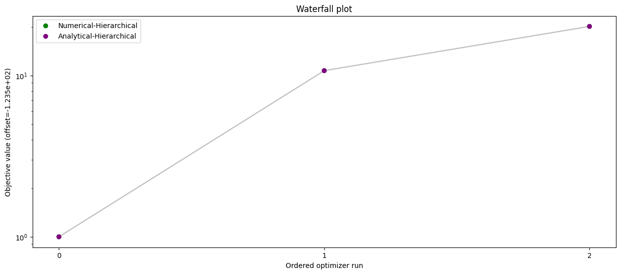
[11]:
# Waterfall plot - analytical vs numerical inner solver
pypesto.visualize.waterfall(
    [result_num, result_ana],
    legends=["Numerical-Hierarchical", "Analytical-Hierarchical"],
    size=(15, 6),
    order_by_id=True,
    colors=np.array(list(map(to_rgba, ("green", "purple")))),
)
[11]:
<Axes: title={'center': 'Waterfall plot'}, xlabel='Ordered optimizer run', ylabel='Objective value (offset=-1.235e+02)'>
[12]:
# Time comparison - analytical vs numerical inner solver
ax = plt.bar(x=[0, 1], height=[time_ana, time_num], color=["purple", "green"])
ax = plt.gca()
ax.set_xticks([0, 1])
ax.set_xticklabels(["Analytical-Hierarchical", "Numerical-Hierarchical"])
ax.set_ylabel("Computation time [s]")
[12]:
Text(0, 0.5, 'Computation time [s]')
Comparison of hierarchical and non-hierarchical optimization
[13]:
# Run standard optimization
start_time = time.time()
result_ord = pypesto.optimize.minimize(problem2, **minimize_kwargs)
print(f"{result_ord.optimize_result.get_for_key('fval')=}")
time_ord = time.time() - start_time
print(f"{time_ord=}")
result_ord.optimize_result.get_for_key('fval')=[168.97019168981913, 542.628899244449, 565.4312610199696]
time_ord=28.25344967842102
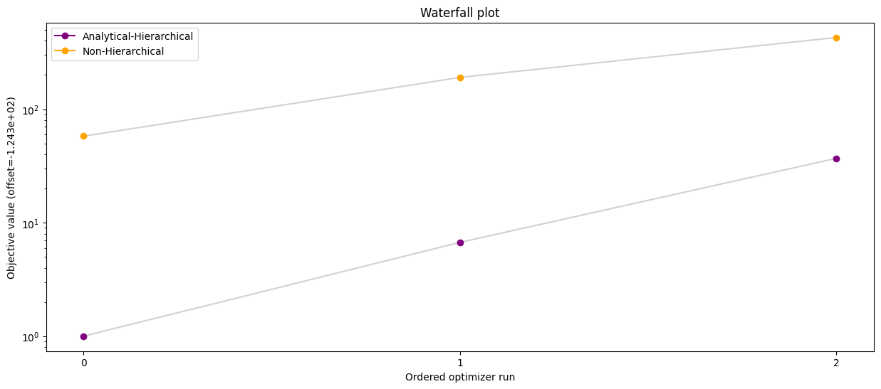
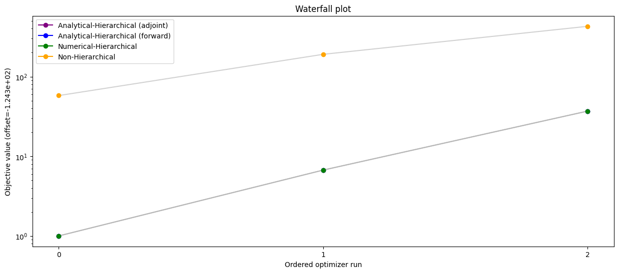
[14]:
# Waterfall plot - hierarchical optimization with analytical inner solver vs standard optimization
pypesto.visualize.waterfall(
    [result_ana, result_ord],
    legends=["Analytical-Hierarchical", "Non-Hierarchical"],
    order_by_id=True,
    colors=np.array(list(map(to_rgba, ("purple", "orange")))),
    size=(15, 6),
)
[14]:
<Axes: title={'center': 'Waterfall plot'}, xlabel='Ordered optimizer run', ylabel='Objective value (offset=-1.235e+02)'>
[15]:
# Time comparison - hierarchical optimization with analytical inner solver vs standard optimization
import matplotlib.pyplot as plt

ax = plt.bar(x=[0, 1], height=[time_ana, time_ord], color=["purple", "orange"])
ax = plt.gca()
ax.set_xticks([0, 1])
ax.set_xticklabels(["Analytical-Hierarchical", "Non-Hierarchical"])
ax.set_ylabel("Computation time [s]")
[15]:
Text(0, 0.5, 'Computation time [s]')
Comparison of hierarchical and non-hierarchical optimization with adjoint and forward sensitivities
[16]:
# Run hierarchical optimization with analytical inner solver and forward sensitivities
start_time = time.time()
problem.objective.calculator.inner_solver = AnalyticalInnerSolver()
problem.objective.amici_solver.set_sensitivity_method(
    SensitivityMethod.forward
)
result_ana_fw = pypesto.optimize.minimize(problem, **minimize_kwargs)
print(f"{result_ana_fw.optimize_result.get_for_key('fval')=}")
time_ana_fw = time.time() - start_time
print(f"{time_ana_fw=}")
result_ana_fw.optimize_result.get_for_key('fval')=[np.float64(124.52978229082845), np.float64(134.23066097095352), np.float64(143.64705349924094)]
time_ana_fw=1.9601945877075195
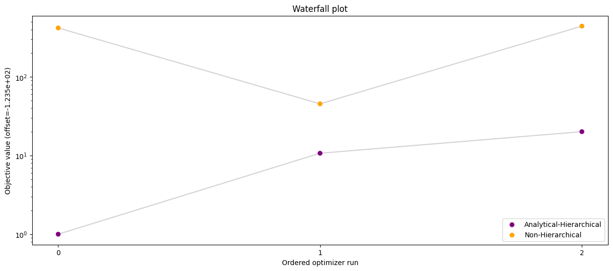
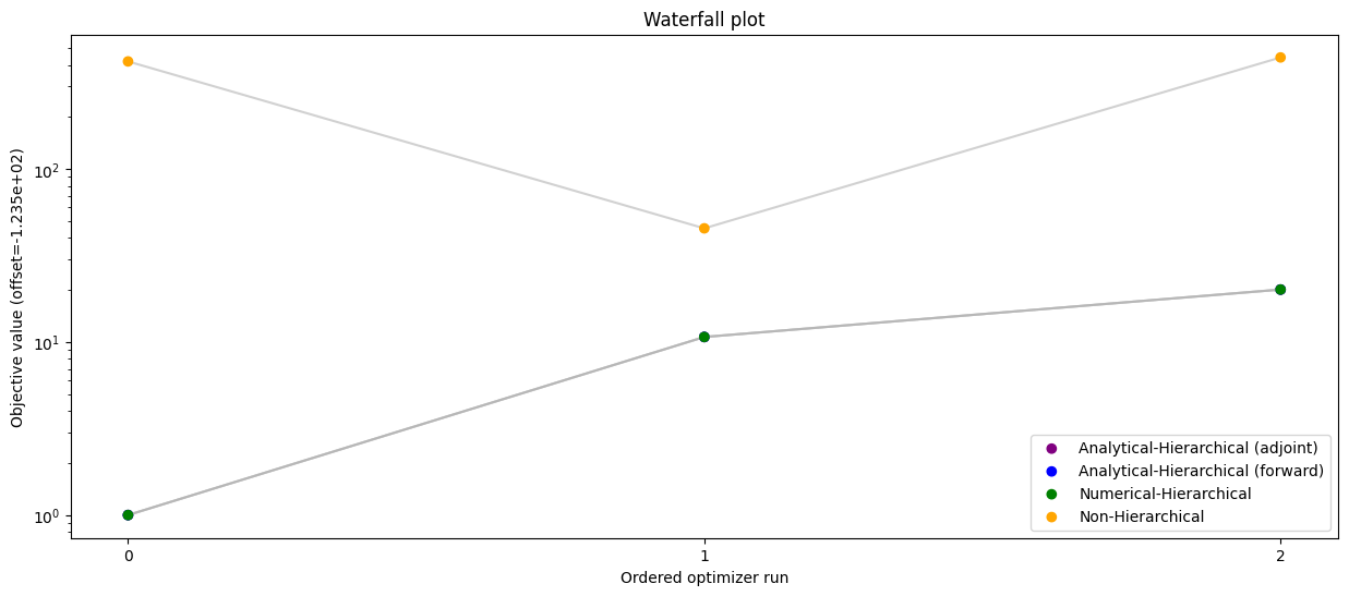
[17]:
# Waterfall plot - compare all scenarios
pypesto.visualize.waterfall(
    [result_ana, result_ana_fw, result_num, result_ord],
    legends=[
        "Analytical-Hierarchical (adjoint)",
        "Analytical-Hierarchical (forward)",
        "Numerical-Hierarchical",
        "Non-Hierarchical",
    ],
    colors=np.array(list(map(to_rgba, ("purple", "blue", "green", "orange")))),
    order_by_id=True,
    size=(15, 6),
)
[17]:
<Axes: title={'center': 'Waterfall plot'}, xlabel='Ordered optimizer run', ylabel='Objective value (offset=-1.235e+02)'>
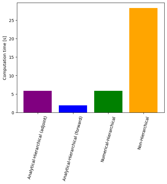
[18]:
# Time comparison of all scenarios
import matplotlib.pyplot as plt

ax = plt.bar(
    x=[0, 1, 2, 3],
    height=[time_ana, time_ana_fw, time_num, time_ord],
    color=["purple", "blue", "green", "orange"],
)
ax = plt.gca()
ax.set_xticks([0, 1, 2, 3])
ax.set_xticklabels(
    [
        "Analytical-Hierarchical (adjoint)",
        "Analytical-Hierarchical (forward)",
        "Numerical-Hierarchical",
        "Non-Hierarchical",
    ]
)
plt.setp(ax.get_xticklabels(), fontsize=10, rotation=75)
ax.set_ylabel("Computation time [s]")
[18]:
Text(0, 0.5, 'Computation time [s]')