RoadRunner in pyPESTO
After going through this notebook, you will be able to…
… create a pyPESTO problem using RoadRunner as a simulator directly from a PEtab problem.
… perform a parameter estimation using pyPESTO with RoadRunner as a simulator, setting advanced simulator features.
[1]:
# install pyPESTO with roadrunner support
# %pip install pypesto[roadrunner,petab] --quiet
[2]:
# import
from pprint import pprint

import matplotlib as mpl
import numpy as np
import petab
from IPython.display import Markdown, display

import pypesto.objective
import pypesto.objective.roadrunner as pypesto_rr
import pypesto.optimize as optimize
import pypesto.petab
import pypesto.visualize as visualize

mpl.rcParams["figure.dpi"] = 100
mpl.rcParams["font.size"] = 18

np.random.seed(1912)


# name of the model that will also be the name of the python module
model_name = "conversion_reaction"
Creating pyPESTO problem from PEtab
The PEtab file format stores all the necessary information to define a parameter estimation problem. This includes the model, the experimental data, the parameters to estimate, and the experimental conditions. Using the pypesto.petab.PetabImporter class, we can create a pyPESTO problem directly from a PEtab problem.
[3]:
petab_yaml = f"./{model_name}/{model_name}.yaml"

petab_problem = petab.Problem.from_yaml(petab_yaml)
importer = pypesto.petab.PetabImporter(
    petab_problem, simulator_type="roadrunner"
)
problem = importer.create_problem()
Visualization table not available. Skipping.
We now have a pyPESTO problem that we can use to perform parameter estimation. We can get some information on the RoadRunnerObjective and access the RoadRunner model.
[4]:
pprint(problem.objective.get_config())
{'roadrunner_instance': '<roadrunner.RoadRunner() { \n'
                        "'this' : 0x5d1e758add90\n"
                        "'modelLoaded' : true\n"
                        "'modelName' : Conversion Reaction 0\n"
                        "'libSBMLVersion' : LibSBML Version: 5.20.5\n"
                        "'jacobianStepSize' : 1e-05\n"
                        "'steadyStateThreshold' : 0.01\n"
                        "'fluxThreshold' : 1e-09\n"
                        "'conservedMoietyAnalysis' : false\n"
                        "'simulateOptions' : \n"
                        '< roadrunner.SimulateOptions() \n'
                        '{ \n'
                        "'this' : 0x5d1e75b75a48, \n"
                        "'reset' : 0,\n"
                        "'structuredResult' : 0,\n"
                        "'copyResult' : 1,\n"
                        "'steps' : 50,\n"
                        "'start' : 0,\n"
                        "'duration' : 5\n"
                        "'output_file' : \n"
                        '}>, \n'
                        "'integrator' : \n"
                        '< roadrunner.Integrator() >\n'
                        '  name: cvode\n'
                        '  settings:\n'
                        '      relative_tolerance: 1e-06\n'
                        '      absolute_tolerance: 1e-12\n'
                        '                   stiff: true\n'
                        '       maximum_bdf_order: 5\n'
                        '     maximum_adams_order: 12\n'
                        '       maximum_num_steps: 20000\n'
                        '       maximum_time_step: 0\n'
                        '       minimum_time_step: 0\n'
                        '       initial_time_step: 0\n'
                        '          multiple_steps: false\n'
                        '      variable_step_size: false\n'
                        '         max_output_rows: 100000\n'
                        '\n'
                        '}>',
 'solver_options': "SolverOptions({'integrator': 'cvode', "
                   "'relative_tolerance': 1e-06, 'absolute_tolerance': 1e-12, "
                   "'maximum_num_steps': 20000})",
 'type': 'RoadRunnerObjective',
 'x_names': ['k1', 'k2']}
[5]:
# direct simulation of the model using roadrunner
sim_res = problem.objective.roadrunner_instance.simulate(
    times=[0, 2.5, 5, 10, 20, 50]
)
pprint(sim_res)
problem.objective.roadrunner_instance.plot();
    time, [A], [B]
 [[    0,   1,   0],
  [  2.5,   1,   0],
  [    5,   1,   0],
  [   10,   1,   0],
  [   20,   1,   0],
  [   50,   1,   0]]
For more details on interacting with the roadrunner instance, we refer to the documentation of libroadrunner. However, we point out that while theoretical possible, we strongly advice against changing the model in that manner.
[6]:
ret = problem.objective(
    petab_problem.get_x_nominal(fixed=False, scaled=True),
    mode="mode_fun",
    return_dict=True,
)
pprint(ret)
{'fval': np.float64(-24.5836745311854),
 'llh': np.float64(24.5836745311854),
 'simulation_results': {'c0':         time,    obs_a
 [[        0,        1],
  [ 0.333333, 0.786907],
  [ 0.666667,  0.65328],
  [        1, 0.569485],
  [  1.33333, 0.516937],
  [  1.66667, 0.483985],
  [        2, 0.463321],
  [  2.33333, 0.450362],
  [  2.66667, 0.442237],
  [        3, 0.437141]]
}}
Optimization
To optimize a problem using a RoadRunner objective, we can set additional solver options for the ODE solver.
[7]:
optimizer = optimize.ScipyOptimizer()

solver_options = pypesto_rr.SolverOptions(
    relative_tolerance=1e-6, absolute_tolerance=1e-12, maximum_num_steps=10000
)
engine = pypesto.engine.SingleCoreEngine()
problem.objective.solver_options = solver_options
[8]:
%%time
result = optimize.minimize(
    problem=problem,
    optimizer=optimizer,
    n_starts=5,  # usually a value >= 100 should be used
    engine=engine,
)
display(Markdown(result.summary()))
Optimization Result
number of starts: 5
best value: -25.356181706742948, id=3
worst value: -25.3561817064364, id=0
number of non-finite values: 0
execution time summary:
Mean execution time: 0.036s
Maximum execution time: 0.045s, id=0
Minimum execution time: 0.024s, id=2
summary of optimizer messages:
Count
Message
5
CONVERGENCE: RELATIVE REDUCTION OF F <= FACTR*EPSMCH
best value found (approximately) 5 time(s)
number of plateaus found: 1
A summary of the best run:
Optimizer Result
optimizer used: <ScipyOptimizer method=L-BFGS-B options={‘maxfun’: 1000}>
message: CONVERGENCE: RELATIVE REDUCTION OF F <= FACTR*EPSMCH
number of evaluations: 105
time taken to optimize: 0.033s
startpoint: [ 1.22253707 -5.01654778]
endpoint: [-0.25416764 -0.60834353]
final objective value: -25.356181706742948
final gradient value: [3.06599191e-04 7.10542732e-06]
CPU times: user 356 ms, sys: 977 μs, total: 357 ms
Wall time: 188 ms
Disclaimer: Currently there are two main things not yet fully supported with roadrunner objectives. One is parallelization of the optimization using MultiProcessEngine. The other is explicit gradients of the objective function. While the former will be added in a near future version, we will show a workaround for the latter, until it is implemented.
Visualization Methods
In order to visualize the optimization, there are a few things possible. For a more extensive explanation we refer to the “getting started” notebook.
[9]:
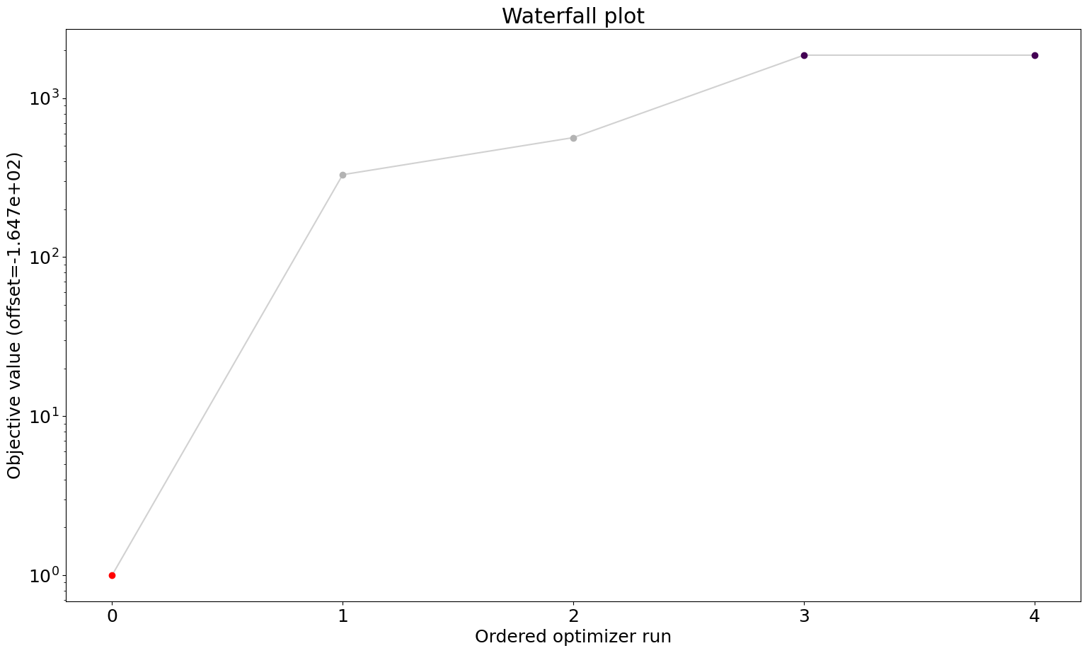
visualize.waterfall(result);
[10]:
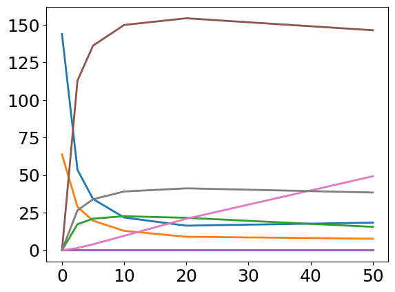
visualize.parameters(result);

[11]:
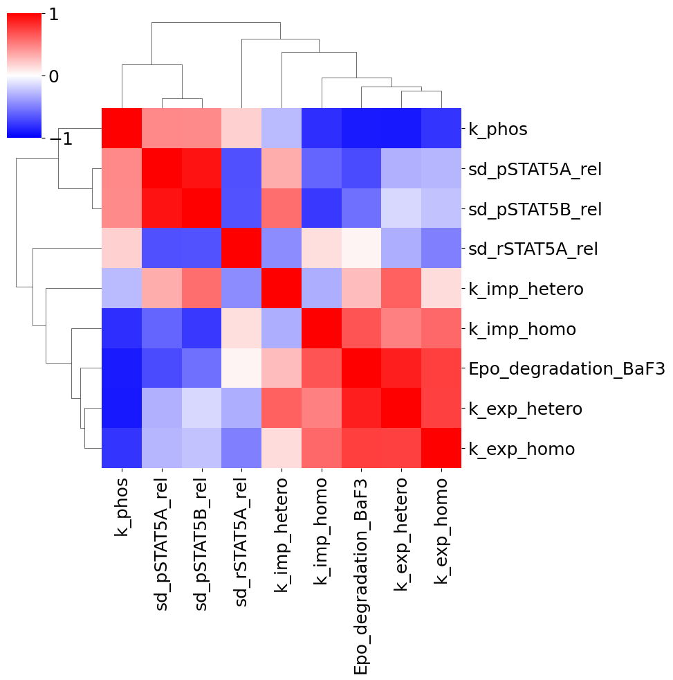
visualize.parameters_correlation_matrix(result);
Sensitivities via finite differences
Some solvers need a way to calculate the sensitivities, which currently RoadRunner Objectives do not suport. For this scenario, we can use the FiniteDifferences objective in pypesto, which wraps a given objective into one, that computes sensitivities via finite differences.
[12]:
# no support for sensitivities
try:
    ret = problem.objective(
        petab_problem.x_nominal_free_scaled,
        mode="mode_fun",
        return_dict=True,
        sensi_orders=(1,),
    )
    pprint(ret)
except ValueError as e:
    pprint(e)
ValueError('This Objective cannot be called with sensi_orders= (1,) and mode=mode_fun.')
[13]:
objective_fd = pypesto.objective.FD(problem.objective)
# support through finite differences
try:
    ret = objective_fd(
        petab_problem.x_nominal_scaled,
        mode="mode_fun",
        return_dict=True,
        sensi_orders=(1,),
    )
    pprint(ret)
except ValueError as e:
    pprint(e)
{'grad': array([-34.93684467, 27.55385614])}