Julia objectives
This notebook demonstrates the application of pyPESTO to objective functions defined in Julia.
pyPESTO’s Julia interface is the class JuliaObjective.
As demonstration example, we use an SIR disease dynamcis model. For simulation, we use DifferentialEquations.jl.
The code consists of multiple functions in the file model_julia/SIR.jl, wrapped in the namespace of a module SIR. We first speficy the reaction network via Catalyst (this is optional, one can also directly start with the differential equations), and then translate them to an ordinary differential equation (ODE) model in OrdinaryDiffEq. Then, we create synthetic observed data with normal noise. After that, we define a quadratic cost function fun (the negative
log-likelihood under an additive normal noise model). We use backwards automatic differentiation via Zygote to derive also the gradient grad (there exist various derivative calculation methods, including forward and adjoint, and continuous and discrete sensitivities, see SciMLSensitivity.jl):
[1]:
from pypesto.objective.julia import display_source_ipython

display_source_ipython("model_julia/SIR.jl")
[1]:
# ODE model of SIR disease dynamics

module SIR

# Install dependencies
import Pkg
Pkg.add(["Catalyst", "OrdinaryDiffEq", "Zygote", "SciMLSensitivity"])

# Define reaction network
using Catalyst: @reaction_network
sir_model = @reaction_network begin
    r1, S + I --> 2I
    r2, I --> R
end r1 r2

# Ground truth parameter
p_true = [0.0001, 0.01]
# Initial state
u0 = [999; 1; 0]
# Time span
tspan = (0.0, 250.0)

# Formulate as ODE problem
using OrdinaryDiffEq: ODEProblem, solve, Tsit5
prob = ODEProblem(sir_model, u0, tspan, p_true)

# True trajectory
sol_true = solve(prob, Tsit5(), saveat=25)

# Observed data
using Random: randn, MersenneTwister
sigma = 40.0
rng = MersenneTwister(1234)
data = sol_true + sigma * randn(rng, size(sol_true))

using SciMLSensitivity: remake

# Define log-likelihood
function fun(p)
    # untransform parameters
    p = 10.0 .^ p
    # simulate
    _prob = remake(prob, p=p)
    sol_sim = solve(_prob, Tsit5(), saveat=25)
    # calculate log-likelihood
    0.5 * (log(2 * pi * sigma^2) + sum((sol_sim .- data).^2) / sigma^2)
end

# Define gradient and Hessian
using Zygote: gradient, hessian

function grad(p)
    gradient(fun, p)[1]
end

function hess(p)
    hessian(fun, p)[1]
end

end  # module
We make the cost function and gradient known to JuliaObjective. Importing module and dependencies, and initializing some operations, can take some time due to pre-processing.
[2]:
import pypesto
from pypesto.objective.julia import JuliaObjective
[3]:
%%time

obj = JuliaObjective(
    module="SIR",
    source_file="model_julia/SIR.jl",
    fun="fun",
    grad="grad",
)
CPU times: user 1min 42s, sys: 3.78 s, total: 1min 46s
Wall time: 1min 48s
That’s it – now we have an objective function that we can simply use in pyPESTO like any other. Internally, it delegates all calls to Julia and translates results.
Comments
Before continuing with the workflow, some comments:
When calling a function for the first time, Julia performs some internal pre-processing. Subsequent function calls are much more efficient.
[4]:
import numpy as np

x = np.array([-4.0, -2.0])

%time print(obj.get_fval(x))
%time print(obj.get_fval(x))
%time print(obj.get_grad(x))
%time print(obj.get_grad(x))
23.12228487889986
CPU times: user 1.36 s, sys: 12.5 ms, total: 1.38 s
Wall time: 1.37 s
23.12228487889986
CPU times: user 208 µs, sys: 11 µs, total: 219 µs
Wall time: 215 µs
[-38.6806348  19.9557434]
CPU times: user 1min 42s, sys: 2.21 s, total: 1min 44s
Wall time: 1min 43s
[-38.6806348  19.9557434]
CPU times: user 1.17 ms, sys: 0 ns, total: 1.17 ms
Wall time: 1.13 ms
The outputs are already numpy arrays (in custom Julia objectives, it needs to be made sure that return objects can be parsed to floats and numpy arrays in Python).
[5]:
type(obj.get_grad(x))
[5]:
numpy.ndarray
Here, we use backward automatic differentiation to calculate the gradient. We can verify its correctness via finite difference checks:
[6]:
from pypesto import FD

fd = FD(obj, grad=True)

fd.get_grad(x)
[6]:
array([-38.75164238, 19.9661208 ])
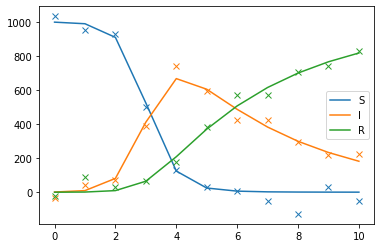
Further, we can use the JuliaObjective.get() function to directly access any variable in the Julia module:
[7]:
sol_true = np.asarray(obj.get("sol_true"))
data = obj.get("data")

import matplotlib.pyplot as plt

for i, label in zip(range(3), ["S", "I", "R"], strict=True):
    plt.plot(sol_true[i], color=f"C{i}", label=label)
    plt.plot(data[i], "x", color=f"C{i}")
plt.legend();
Inference problem
Let us define an inference problem by specifying parameter bounds. Note that we use a log10-transformation of parameters in fun.
[8]:
from pypesto import Problem

# parameter boundaries
lb, ub = [-5.0, -3.0], [-3.0, -1.0]

# estimation problem
problem = Problem(obj, lb=lb, ub=ub)
Optimization
Let us perform an optimization:
[9]:
%%time

# optimize
from pypesto import optimize

result = optimize.minimize(problem)
100%|██████████████████████████████████████████████████████████████| 100/100 [00:01<00:00, 77.83it/s]
CPU times: user 1.38 s, sys: 88.2 ms, total: 1.47 s
Wall time: 1.47 s
The objective function evaluations are quite fast!
We can also use parallelization, by passing a pypesto.engine.MultiProcessEngine to the minimize function.
[10]:
%%time

from pypesto.engine import MultiProcessEngine

engine = MultiProcessEngine()
result = optimize.minimize(problem, engine=engine, n_starts=100)
Engine set up to use up to 8 processes in total. The number was automatically determined and might not be appropriate on some systems.
2022-09-07 00:49:47,222 - pypesto.engine.multi_process - WARNING - Engine set up to use up to 8 processes in total. The number was automatically determined and might not be appropriate on some systems.
Performing parallel task execution on 8 processes.
2022-09-07 00:49:47,233 - pypesto.engine.multi_process - INFO - Performing parallel task execution on 8 processes.
100%|█████████████████████████████████████████████████████████████| 100/100 [00:00<00:00, 130.42it/s]
CPU times: user 285 ms, sys: 177 ms, total: 462 ms
Wall time: 1.73 s
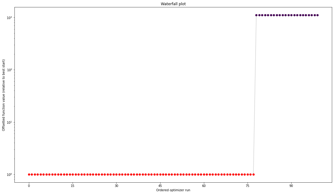
[11]:
from pypesto import visualize

visualize.waterfall(result);
Sampling
Last, let us perform sampling from the log-posterior with implicitly defined uniform prior via the parameter bounds:
[12]:
%%time

from pypesto import sample

sampler = sample.AdaptiveParallelTemperingSampler(
    internal_sampler=sample.AdaptiveMetropolisSampler(), n_chains=3
)

result = sample.sample(
    problem, n_samples=10000, sampler=sampler, result=result
)
100%|████████████████████████████████████████████████████████| 10000/10000 [00:08<00:00, 1234.51it/s]
Elapsed time: 8.135626907000017
2022-09-07 00:49:57,692 - pypesto.sample.sample - INFO - Elapsed time: 8.135626907000017
CPU times: user 7.87 s, sys: 320 ms, total: 8.18 s
Wall time: 8.15 s
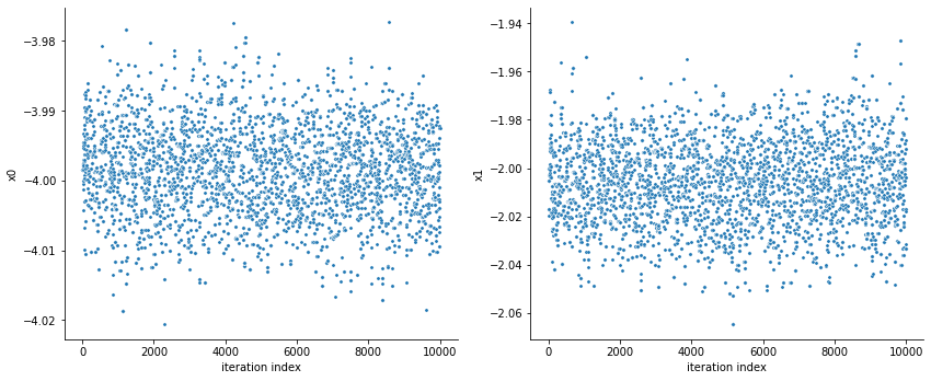
[13]:
pypesto.sample.geweke_test(result)
visualize.sampling_parameter_traces(
    result, use_problem_bounds=False, size=(12, 5)
);
Geweke burn-in index: 0
2022-09-07 00:49:57,807 - pypesto.sample.diagnostics - INFO - Geweke burn-in index: 0
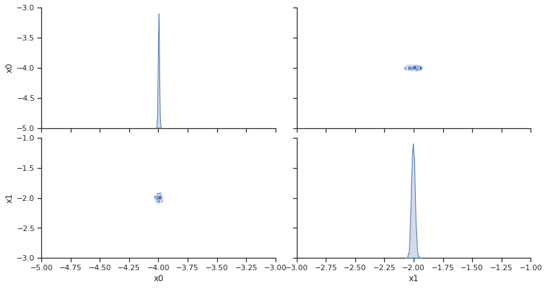
[14]:
visualize.sampling_scatter(result, size=[13, 6]);