Model import using the PEtab format

In this notebook, we illustrate how to use pyPESTO together with PEtab and AMICI. The notebook first details the individual steps of the import and the creation of the objective function. Note that those steps can be summarised, demonstrated at the end of the ‘Import’ section. After that, optimization and visualisation are showcased. We employ models from the benchmark collection, which we first download:

# install if not done yet
# !apt install libatlas-base-dev swig
# %pip install pypesto[amici,petab] --quiet
# %pip install git+https://github.com/Benchmarking-Initiative/Benchmark-Models-PEtab.git@master#subdirectory=src/python --quiet

import os
from pprint import pprint

import benchmark_models_petab as models
import numpy as np
import petab

import pypesto.optimize as optimize
import pypesto.petab
import pypesto.visualize as visualize

Import

Manage PEtab model

A PEtab problem comprises all the information on the model, the data and the parameters to perform parameter estimation. We import a model as a petab.Problem.

# a collection of models that can be simulated

# model_name = "Zheng_PNAS2012"
model_name = "Boehm_JProteomeRes2014"
# model_name = "Fujita_SciSignal2010"
# model_name = "Sneyd_PNAS2002"
# model_name = "Borghans_BiophysChem1997"
# model_name = "Elowitz_Nature2000"
# model_name = "Crauste_CellSystems2017"
# model_name = "Lucarelli_CellSystems2018"
# model_name = "Schwen_PONE2014"
# model_name = "Blasi_CellSystems2016"

# the yaml configuration file links to all needed files
yaml_config = os.path.join(models.MODELS_DIR, model_name, model_name + ".yaml")

# create a petab problem
petab_problem = petab.Problem.from_yaml(yaml_config)

Import model to AMICI

In order to import the model into pyPESTO, we additionally need a simulator. We can specify the simulator through the simulator_type argument. Supported simulators are e.g.amici and roadrunner. We will use AMICI as our example simulator. Therefore, we create a pypesto.PetabImporter from the problem. The importer itself creates a pypesto.petab.Factory, which is used to create the AMICI objective and model.

importer = pypesto.petab.PetabImporter(petab_problem, simulator_type="amici")
factory = importer.create_objective_creator()

model = factory.create_model(verbose=False)

# some model properties
print("Model parameters:", list(model.getParameterIds()), "\n")
print("Model const parameters:", list(model.getFixedParameterIds()), "\n")
print("Model outputs:   ", list(model.getObservableIds()), "\n")
print("Model states:    ", list(model.getStateIds()), "\n")

Compiling amici model to folder /home/docs/checkouts/readthedocs.org/user_builds/pypesto/checkouts/latest/doc/example/amici_models/0.30.0/Boehm_JProteomeRes2014.

Model parameters: ['Epo_degradation_BaF3', 'k_exp_hetero', 'k_exp_homo', 'k_imp_hetero', 'k_imp_homo', 'k_phos', 'noiseParameter1_pSTAT5A_rel', 'noiseParameter1_pSTAT5B_rel', 'noiseParameter1_rSTAT5A_rel']

Model const parameters: ['ratio', 'specC17']

Model outputs:    ['pSTAT5A_rel', 'pSTAT5B_rel', 'rSTAT5A_rel']

Model states:     ['STAT5A', 'STAT5B', 'pApB', 'pApA', 'pBpB', 'nucpApA', 'nucpApB', 'nucpBpB']

Create objective function

To perform parameter estimation, we need to define an objective function, which integrates the model, data, and noise model defined in the PEtab problem.

Creating the objective from PEtab with default settings can be done in as little as two lines.

importer = pypesto.petab.PetabImporter.from_yaml(yaml_config, simulator_type="amici")
problem = importer.create_problem()  # creating the problem from the importer. The objective can be found at problem.objective

If you need more flexibility, e.g., to define whether you need residuals of the objective function, what sensitivities you want to use, or fix certain parameters, you can also create the problem from a customized objective:

import libsbml

converter_config = libsbml.SBMLLocalParameterConverter().getDefaultProperties()
petab_problem.sbml_document.convert(converter_config)

factory = importer.create_objective_creator()
obj = factory.create_objective()

# for some models, hyperparameters need to be adjusted
# obj.amici_solver.setMaxSteps(10000)
# obj.amici_solver.setRelativeTolerance(1e-7)
# obj.amici_solver.setAbsoluteTolerance(1e-7)

We can request variable derivatives via sensi_orders, function values or residuals as specified via mode. Passing return_dict, we obtain the direct result of the AMICI simulation.

ret = obj(
    petab_problem.x_nominal_scaled,
    mode="mode_fun",
    sensi_orders=(0, 1),
    return_dict=True,
)
pprint(ret)

{'fval': 138.22199623526868,
 'grad': array([ 2.20322414e-02,  5.53227517e-02,  5.78778194e-03,  5.40047566e-03,
       -4.51595808e-05,  7.91499745e-03,  0.00000000e+00,  1.07840690e-02,
        2.40397699e-02,  1.91925824e-02,  0.00000000e+00]),
 'rdatas': [<ReturnDataView(id='model1_data1', status=AMICI_SUCCESS)>]}

The problem defined in PEtab also defines the fixed parameters and parameter bounds. This information is contained in a pypesto.Problem.

problem = importer.create_problem(obj)

In particular, the problem accounts for the fixation of parameters.

print(f"{problem.x_fixed_indices=}")
print(f"{problem.x_free_indices=}")

problem.x_fixed_indices=[6, 10]
problem.x_free_indices=[0, 1, 2, 3, 4, 5, 7, 8, 9]

The problem creates a copy of the objective function that takes into account the fixed parameters. The objective function is able to calculate function values and derivatives. A finite difference checks whether the computed gradient is accurate:

objective = problem.objective
fval, gradient = objective(
    petab_problem.x_nominal_free_scaled, sensi_orders=(0, 1)
)
print(f"{fval=}\n{gradient=}")

fval=138.22199623526868
gradient=array([ 2.20322414e-02,  5.53227517e-02,  5.78778194e-03,  5.40047566e-03,
       -4.51595808e-05,  7.91499745e-03,  1.07840690e-02,  2.40397699e-02,
        1.91925824e-02])

eps = 1e-4


def fd(x):
    grad = np.zeros_like(x)
    j = 0
    for i, _xi in enumerate(x):
        mask = np.zeros_like(x)
        mask[i] += eps
        valinc, _ = objective(x + mask, sensi_orders=(0, 1))
        valdec, _ = objective(x - mask, sensi_orders=(0, 1))
        grad[j] = (valinc - valdec) / (2 * eps)
        j += 1
    return grad


fdval = fd(petab_problem.x_nominal_free_scaled)
for i, (g, f) in enumerate(zip(gradient, fdval)):
    print(f"{i=}: {g=:9f},\t{f=:9f},\t{g - f=:9f}")
print(f"l2 difference: {np.linalg.norm(gradient - fdval):.2e}")

i=0: g= 0.022032,       f= 0.032126,    g - f=-0.010094
i=1: g= 0.055323,       f= 0.065958,    g - f=-0.010635
i=2: g= 0.005788,       f=-0.001403,    g - f= 0.007191
i=3: g= 0.005400,       f=-0.001799,    g - f= 0.007200
i=4: g=-0.000045,       f=-0.014022,    g - f= 0.013977
i=5: g= 0.007915,       f= 0.010970,    g - f=-0.003055
i=6: g= 0.010784,       f= 0.010783,    g - f= 0.000001
i=7: g= 0.024040,       f= 0.024038,    g - f= 0.000001
i=8: g= 0.019193,       f= 0.019191,    g - f= 0.000001
l2 difference: 2.29e-02

Run optimization

Given the problem, we can perform optimization. We can specify an optimizer to use, and a parallelization engine to speed things up.

optimizer = optimize.ScipyOptimizer()

# engine = pypesto.engine.SingleCoreEngine()
engine = pypesto.engine.MultiProcessEngine()

# do the optimization
result = optimize.minimize(
    problem=problem, optimizer=optimizer, n_starts=10, engine=engine
)

Engine will use up to 2 processes (= CPU count).

Dealing with function evaluations at the initial point

It is quite common in real applications that the objective function is evaluable at every point in parameter space. Therefore, some local optimizations may fail directly at their initial point. Such results are usually not very informative and would be discarded. To directly discard such initial points, we can select a startpoint method that will resample starting points if the objective function (check_fval) or its gradient (check_grad) are non-finite:

problem = importer.create_problem(
    startpoint_kwargs={"check_fval": True, "check_grad": True}
)

Visualize

The results are contained in a pypesto.Result object. It contains e.g., the optimal function values.

result.optimize_result.fval

[145.7594115389956,
 149.58783205317957,
 150.6774670046416,
 150.6809917097522,
 154.7331367600722,
 249.74581758184635,
 249.74599476339557,
 249.74599651484056,
 249.7459974414443,
 249.74599744208615]

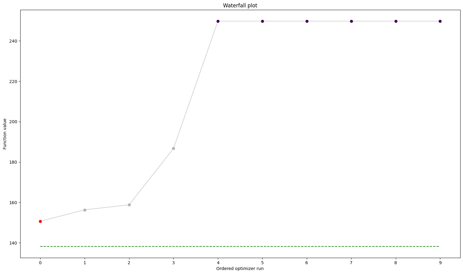
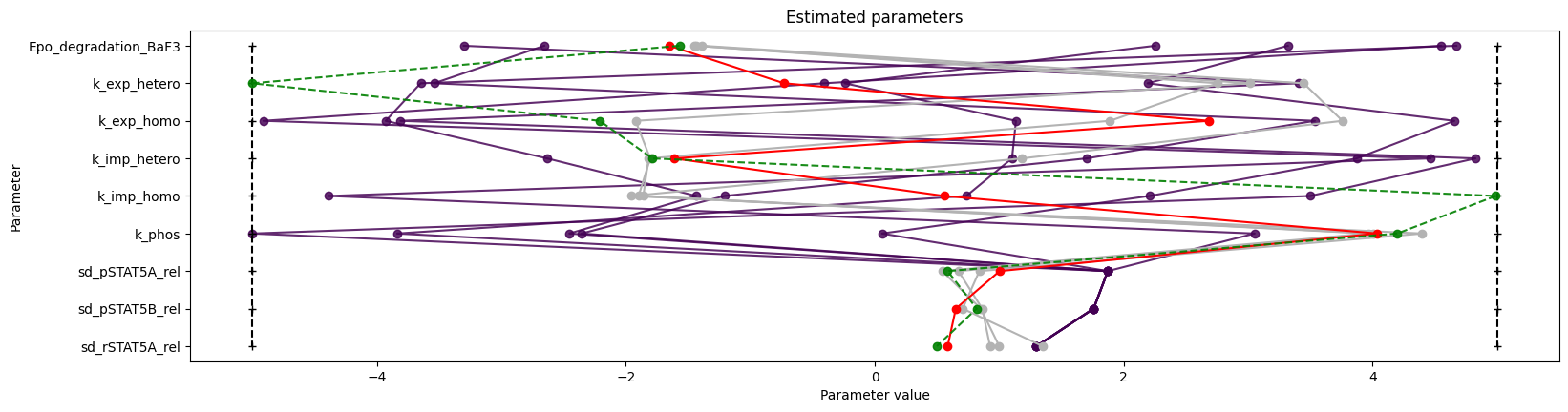
We can use the standard pyPESTO plotting routines to visualize and analyze the results.

ref = visualize.create_references(
    x=petab_problem.x_nominal_scaled, fval=obj(petab_problem.x_nominal_scaled)
)

visualize.waterfall(result, reference=ref, scale_y="lin")
visualize.parameters(result, reference=ref);

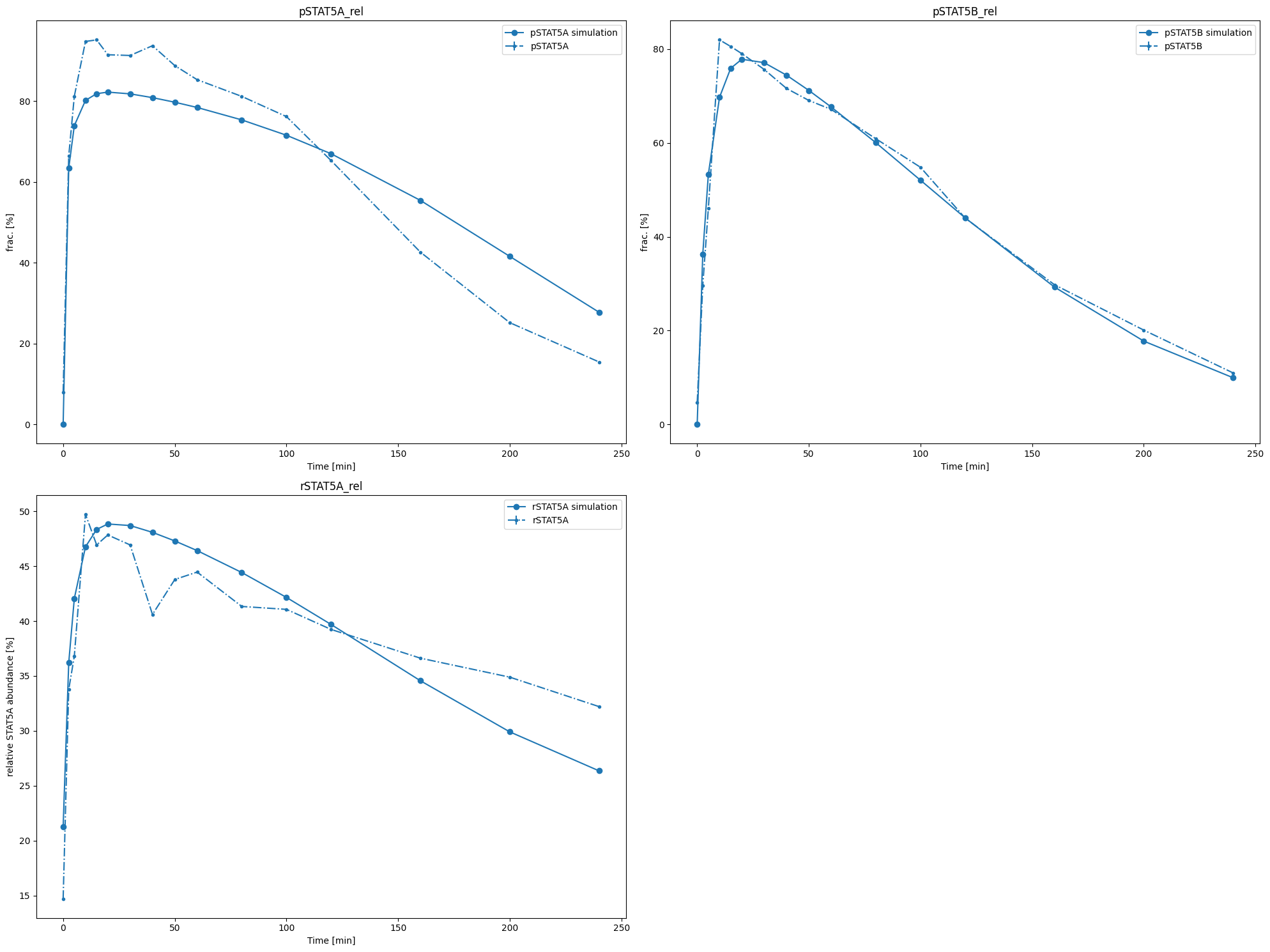
We can also conveniently visualize the model fit. This plots the petab visualization using optimized parameters.

# we need to explicitly import the method
from pypesto.visualize.model_fit import visualize_optimized_model_fit

visualize_optimized_model_fit(
    petab_problem=petab_problem, result=result, pypesto_problem=problem
);