A sampler study
In this notebook, we perform a short study of how various samplers implemented in pyPESTO perform.
[1]:
# install if not done yet
# !apt install libatlas-base-dev swig
# %pip install pypesto[amici,petab,pymc,emcee] --quiet
The pipeline
First, we show a typical workflow, fully integrating the samplers with a PEtab problem, using a toy example of a conversion reaction.
[2]:
import numpy as np
import petab

import pypesto
import pypesto.optimize as optimize
import pypesto.petab
import pypesto.sample as sample
import pypesto.visualize as visualize

np.random.seed(0)

# import to petab
petab_problem = petab.Problem.from_yaml(
    "conversion_reaction/conversion_reaction.yaml"
)
# import to pypesto
importer = pypesto.petab.PetabImporter(petab_problem)
# create problem
problem = importer.create_problem(verbose=False)
Visualization table not available. Skipping.
2026-03-18 12:55:22.838 - amici.sim.sundials.petab.v1._parameter_mapping - DEBUG - PEtab mapping: ({}, {'k1': 'k1', 'k2': 'k2'}, {}, {'k1': 'log', 'k2': 'log'})
2026-03-18 12:55:22.838 - amici.sim.sundials.petab.v1._parameter_mapping - DEBUG - Fixed parameters pre-equilibration: {}
2026-03-18 12:55:22.839 - amici.sim.sundials.petab.v1._parameter_mapping - DEBUG - Fixed parameters simulation: {}
2026-03-18 12:55:22.840 - amici.sim.sundials.petab.v1._parameter_mapping - DEBUG - Variable parameters pre-equilibration: {}
2026-03-18 12:55:22.840 - amici.sim.sundials.petab.v1._parameter_mapping - DEBUG - Variable parameters simulation: {'k1': 'k1', 'k2': 'k2'}
2026-03-18 12:55:22.840 - amici.sim.sundials.petab.v1._parameter_mapping - DEBUG - Merged: {'k1': 'k1', 'k2': 'k2'}
[3]:
problem.x_names
[3]:
['k1', 'k2']
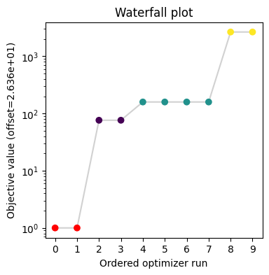
Commonly, as a first step, optimization is performed, in order to find good parameter point estimates.
[4]:
result = optimize.minimize(problem, n_starts=10, filename=None)
[5]:
visualize.waterfall(result, size=(4, 4));
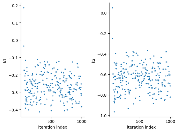
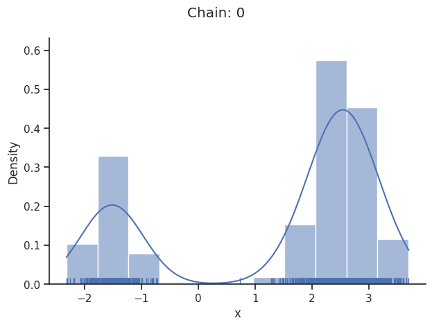
Next, we perform sampling. Here, we employ a pypesto.sample.AdaptiveParallelTemperingSampler sampler, which runs Markov Chain Monte Carlo (MCMC) chains on different temperatures. For each chain, we employ a pypesto.sample.AdaptiveMetropolisSampler. For more on the samplers see below or the API documentation.
[6]:
sampler = sample.AdaptiveParallelTemperingSampler(
    internal_sampler=sample.AdaptiveMetropolisSampler(),
    n_chains=3,
)
Initializing betas with "near-exponential decay".
For the actual sampling, we call the pypesto.sample.sample function. By passing the result object to the function, the previously found global optimum is used as starting point for the MCMC sampling.
[7]:
%%time
result = sample.sample(
    problem, n_samples=1000, sampler=sampler, result=result, filename=None
)
Initializing parallel chains with a combination of the starting point and prior samples with weight: 0.9.
Elapsed time: 1.2670609079999995
CPU times: user 1.23 s, sys: 42.5 ms, total: 1.28 s
Wall time: 1.27 s
When the sampling is finished, we can analyse our results. A first thing to do is to analyze the sampling burn-in:
[8]:
sample.geweke_test(result)
Geweke burn-in index: 50
[8]:
np.int64(50)
pyPESTO provides functions to analyse both the sampling process as well as the obtained sampling result. Visualizing the traces e.g. allows to detect burn-in phases, or fine-tune hyperparameters. First, the parameter trajectories can be visualized:
[9]:
ax = visualize.sampling_parameter_traces(result, use_problem_bounds=False)
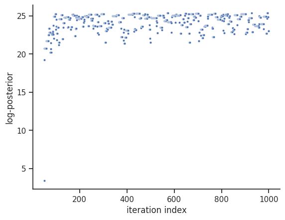
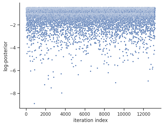
Next, also the log posterior trace can be visualized:
[10]:
ax = visualize.sampling_fval_traces(result)
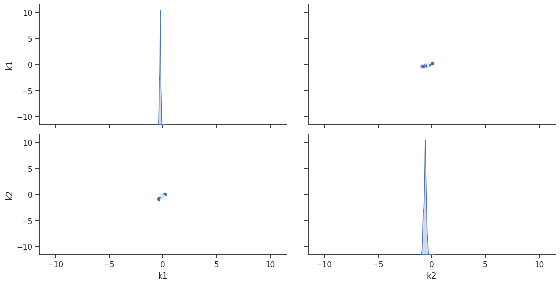
To visualize the result, there are various options. The scatter plot shows histograms of 1-dim parameter marginals and scatter plots of 2-dimensional parameter combinations:
[11]:
ax = visualize.sampling_scatter(result, size=[13, 6])
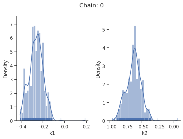
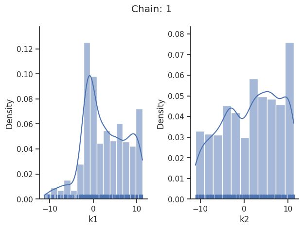
sampling_1d_marginals allows to plot e.g. kernel density estimates or histograms (internally using seaborn):
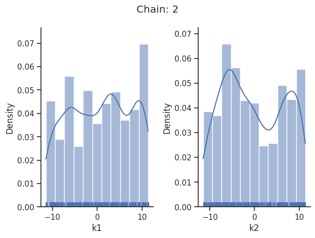
[12]:
for i_chain in range(len(result.sample_result.betas)):
    visualize.sampling_1d_marginals(
        result, i_chain=i_chain, suptitle=f"Chain: {i_chain}"
    )
That’s it for the moment on using the sampling pipeline.
1-dim test problem
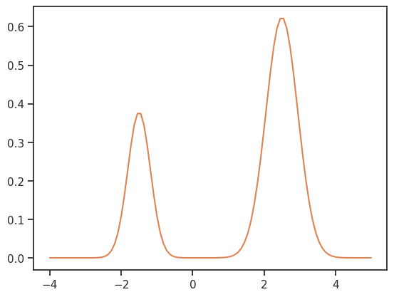
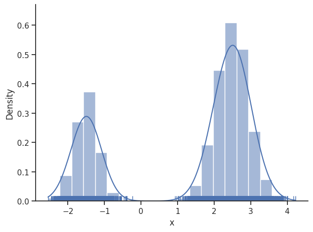
To compare and test the various implemented samplers, we first study a 1-dimensional test problem of a gaussian mixture density, together with a flat prior.
[13]:
import seaborn as sns
from scipy.stats import multivariate_normal

import pypesto
import pypesto.sample as sample
import pypesto.visualize as visualize


def density(x):
    return 0.3 * multivariate_normal.pdf(
        x, mean=-1.5, cov=0.1
    ) + 0.7 * multivariate_normal.pdf(x, mean=2.5, cov=0.2)


def nllh(x):
    return -np.log(density(x))


objective = pypesto.Objective(fun=nllh)
problem = pypesto.Problem(objective=objective, lb=-4, ub=5, x_names=["x"])
The likelihood has two separate modes:
[14]:
xs = np.linspace(-4, 5, 100)
ys = [density(x) for x in xs]

ax = sns.lineplot(x=xs, y=ys, color="C1")
Metropolis sampler
For this problem, let us try out the simplest sampler, the pypesto.sample.MetropolisSampler.
[15]:
sampler = sample.MetropolisSampler({"std": 0.5})
result = sample.sample(
    problem, 1e3, sampler, x0=np.array([0.5]), filename=None
)
Elapsed time: 0.1908825640000007
[16]:
sample.geweke_test(result)
ax = visualize.sampling_1d_marginals(result)
ax[0][0].plot(xs, ys)
Geweke burn-in index: 100
[16]:
[<matplotlib.lines.Line2D at 0x7fb438d1c410>]
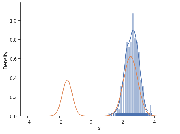
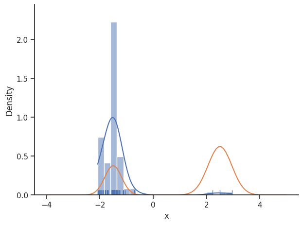
The obtained posterior does not accurately represent the distribution, often only capturing one mode. This is because it is hard for the Markov chain to jump between the distribution’s two modes. This can be fixed by choosing a higher proposal variation std:
[17]:
sampler = sample.MetropolisSampler({"std": 1})
result = sample.sample(
    problem, 1e3, sampler, x0=np.array([0.5]), filename=None
)
Elapsed time: 0.1973530960000005
[18]:
sample.geweke_test(result)
ax = visualize.sampling_1d_marginals(result)
ax[0][0].plot(xs, ys)
Geweke burn-in index: 900
[18]:
[<matplotlib.lines.Line2D at 0x7fb438db3110>]
In general, MCMC have difficulties exploring multimodel landscapes. One way to overcome this is to used parallel tempering. There, various chains are run, lifting the densities to different temperatures. At high temperatures, proposed steps are more likely to get accepted and thus jumps between modes are more likely.
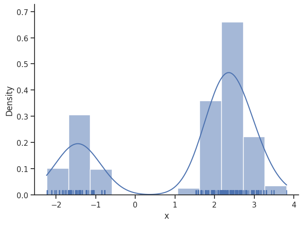
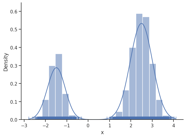
Parallel tempering sampler
In pyPESTO, the most basic parallel tempering algorithm is the pypesto.sample.ParallelTemperingSampler. It takes an internal_sampler parameter, to specify what sampler to use for performing sampling the different chains. Further, we can directly specify what inverse temperatures betas to use. When not specifying the betas explicitly, but just the number of chains n_chains, an established near-exponential decay scheme is used.
[19]:
sampler = sample.ParallelTemperingSampler(
    internal_sampler=sample.MetropolisSampler(), betas=[1, 1e-1, 1e-2]
)
result = sample.sample(
    problem, 1e3, sampler, x0=np.array([0.5]), filename=None
)
Initializing parallel chains with a combination of the starting point and prior samples with weight: 0.9.
Elapsed time: 0.6994294679999999
[20]:
sample.geweke_test(result)
for i_chain in range(len(result.sample_result.betas)):
    visualize.sampling_1d_marginals(
        result, i_chain=i_chain, suptitle=f"Chain: {i_chain}"
    )
Geweke burn-in index: 50
Of interest is here finally the first chain at index i_chain=0, which approximates the posterior well.
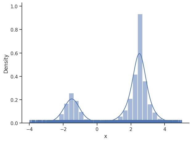
Adaptive Metropolis sampler
The problem of having to specify the proposal step variation manually can be overcome by using the pypesto.sample.AdaptiveMetropolisSampler, which iteratively adjusts the proposal steps to the function landscape.
[21]:
sampler = sample.AdaptiveMetropolisSampler()
result = sample.sample(
    problem, 1e3, sampler, x0=np.array([0.5]), filename=None
)
Elapsed time: 0.2505733079999999
[22]:
sample.geweke_test(result)
ax = visualize.sampling_1d_marginals(result)
Geweke burn-in index: 100
Adaptive parallel tempering sampler
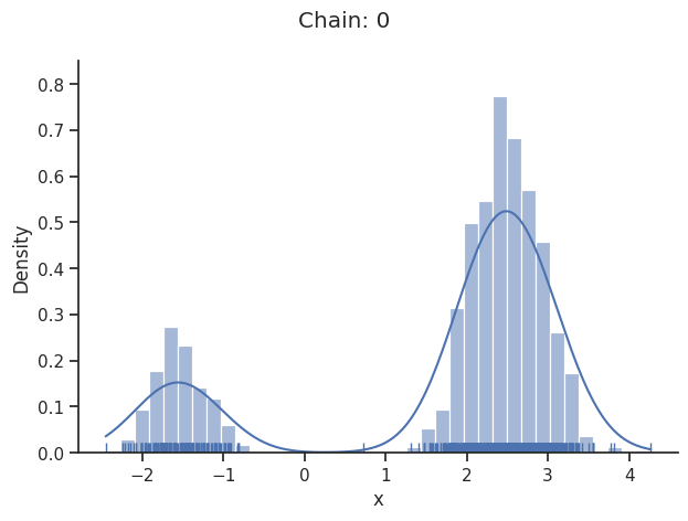
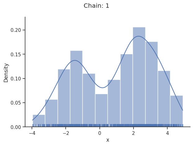
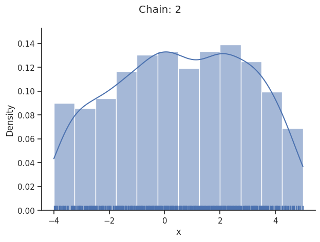
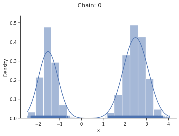
The pypesto.sample.AdaptiveParallelTemperingSampler iteratively adjusts the temperatures to obtain good swapping rates between chains.
[23]:
sampler = sample.AdaptiveParallelTemperingSampler(
    internal_sampler=sample.AdaptiveMetropolisSampler(), n_chains=3
)
result = sample.sample(
    problem, 1e3, sampler, x0=np.array([0.5]), filename=None
)
Initializing betas with "near-exponential decay".
Initializing parallel chains with a combination of the starting point and prior samples with weight: 0.9.
Elapsed time: 0.7350516030000005
[24]:
sample.geweke_test(result)
for i_chain in range(len(result.sample_result.betas)):
    visualize.sampling_1d_marginals(
        result, i_chain=i_chain, suptitle=f"Chain: {i_chain}"
    )
Geweke burn-in index: 0
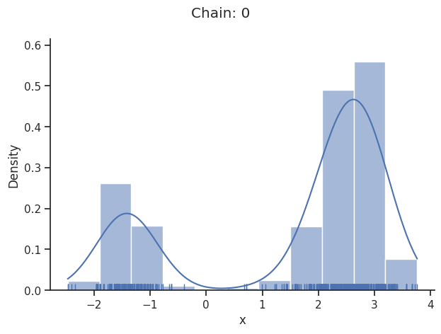
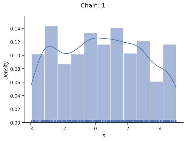
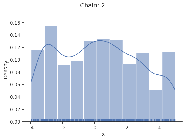
[25]:
result.sample_result.betas
[25]:
array([1.00000000e+00, 3.35271615e-02, 2.00000000e-05])
Pymc sampler
[26]:
from pypesto.sample.pymc import PymcSampler

sampler = PymcSampler()
result = sample.sample(
    problem, 1e3, sampler, x0=np.array([0.5]), filename=None
)
Sequential sampling (1 chains in 1 job)
Slice: [x]
Sampling 1 chain for 1_000 tune and 1_000 draw iterations (1_000 + 1_000 draws total) took 3 seconds.
Only one chain was sampled, this makes it impossible to run some convergence checks
Elapsed time: 3.6848919130000013
[27]:
sample.geweke_test(result)
for i_chain in range(len(result.sample_result.betas)):
    visualize.sampling_1d_marginals(
        result, i_chain=i_chain, suptitle=f"Chain: {i_chain}"
    )
Geweke burn-in index: 0
If not specified, pymc chooses an adequate sampler automatically.
Emcee sampler
[28]:
sampler = sample.EmceeSampler(nwalkers=10, run_args={"progress": True})
result = sample.sample(
    problem, int(1e3), sampler, x0=np.array([0.5]), filename=None
)
Elapsed time: 1.9375258739999985
[29]:
np.array([sampler.sampler.get_log_prob(flat=True)]).shape
[29]:
(1, 10000)
[30]:
sample.geweke_test(result)
for i_chain in range(len(result.sample_result.betas)):
    visualize.sampling_1d_marginals(
        result, i_chain=i_chain, suptitle=f"Chain: {i_chain}"
    )
Geweke burn-in index: 500
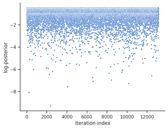
dynesty sampler
The dynesty package provides nested and dynamic nested samplers. These differ from some of the other samplers that pyPESTO interfaces with. For example, it doesn’t make sense to request a certain number of samples. Instead, the sampler runs until stopping criteria have been met.
[31]:
sampler = sample.DynestySampler(objective_type="negloglike")
result = sample.sample(
    problem=problem,
    n_samples=None,
    sampler=sampler,
    filename=None,
)
Assuming 'prior_transform' is correctly specified. If 'x_priors' is not uniform, 'prior_transform' has to be adjusted accordingly.
Elapsed time: 19.104174712000003
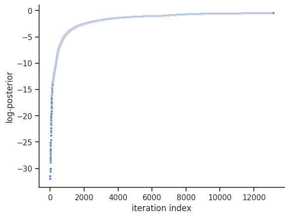
Another difference is that there is no burn-in so, unlike for some other pyPESTO sampler results, the Geweke test is not applied here, and the chain will not appear to be converged. However, by default, pyPESTO returns samples that have been resampled to appear like converged chains from MCMC sampling.
[32]:
visualize.sampling_1d_marginals(result)
visualize.sampling_fval_traces(result, full_trace=True)
/home/docs/checkouts/readthedocs.org/user_builds/pypesto/envs/latest/lib/python3.13/site-packages/pypesto/visualize/sampling.py:1291: UserWarning: Burn in index not found in the results, the full chain will be shown.
You may want to use, e.g., `pypesto.sample.geweke_test`.
  nr_params, params_fval, theta_lb, theta_ub, param_names = get_data_to_plot(
/home/docs/checkouts/readthedocs.org/user_builds/pypesto/envs/latest/lib/python3.13/site-packages/pypesto/visualize/sampling.py:78: UserWarning: Burn in index not found in the results, the full chain will be shown.
You may want to use, e.g., `pypesto.sample.geweke_test`.
  _, params_fval, _, _, _ = get_data_to_plot(
[32]:
<Axes: xlabel='iteration index', ylabel='log-posterior'>
The internal dynesty sampler can be saved and restored, for post-sampling analysis. For example, pyPESTO stores resampled MCMC-like samples from the dynesty sampler by default. The following code shows how to save and load the internal dynesty sampler, to facilitate post-sampling analysis of both the resampled and original chains. N.B.: when working across different computers, you might prefer to work with the raw sample results via pypesto.sample.dynesty.save_raw_results and
load_raw_results. First, we save the internal sampler.
[33]:
sampler.save_internal_sampler("dynesty.dill")
Next, we load the internal sampler into some DynestySampler object, then set the sample_result of some pyPESTO result to the original samples.
[34]:
dummy_sampler = sample.DynestySampler()
dummy_sampler.restore_internal_sampler("dynesty.dill")
dummy_result = pypesto.Result(problem=problem)

dummy_result.sample_result = dummy_sampler.get_original_samples()
visualize.sampling_1d_marginals(dummy_result)
visualize.sampling_fval_traces(dummy_result)
Assuming 'prior_transform' is correctly specified. If 'x_priors' is not uniform, 'prior_transform' has to be adjusted accordingly.
/home/docs/checkouts/readthedocs.org/user_builds/pypesto/envs/latest/lib/python3.13/site-packages/pypesto/visualize/sampling.py:1291: UserWarning: Burn in index not found in the results, the full chain will be shown.
You may want to use, e.g., `pypesto.sample.geweke_test`.
  nr_params, params_fval, theta_lb, theta_ub, param_names = get_data_to_plot(
/home/docs/checkouts/readthedocs.org/user_builds/pypesto/envs/latest/lib/python3.13/site-packages/pypesto/visualize/sampling.py:78: UserWarning: Burn in index not found in the results, the full chain will be shown.
You may want to use, e.g., `pypesto.sample.geweke_test`.
  _, params_fval, _, _, _ = get_data_to_plot(
[34]:
<Axes: xlabel='iteration index', ylabel='log-posterior'>
We then set the sample_result of the dummy_result back to MCMC-like resampled samples.
[35]:
dummy_result.sample_result = dummy_sampler.get_samples()
visualize.sampling_1d_marginals(dummy_result)
visualize.sampling_fval_traces(dummy_result)
/home/docs/checkouts/readthedocs.org/user_builds/pypesto/envs/latest/lib/python3.13/site-packages/pypesto/visualize/sampling.py:1291: UserWarning: Burn in index not found in the results, the full chain will be shown.
You may want to use, e.g., `pypesto.sample.geweke_test`.
  nr_params, params_fval, theta_lb, theta_ub, param_names = get_data_to_plot(
/home/docs/checkouts/readthedocs.org/user_builds/pypesto/envs/latest/lib/python3.13/site-packages/pypesto/visualize/sampling.py:78: UserWarning: Burn in index not found in the results, the full chain will be shown.
You may want to use, e.g., `pypesto.sample.geweke_test`.
  _, params_fval, _, _, _ = get_data_to_plot(
[35]:
<Axes: xlabel='iteration index', ylabel='log-posterior'>
This sampler supports parallelization, see the dynesty documentation for more details: https://dynesty.readthedocs.io
An example of doing this via pyPESTO is given below
import multiprocessing
import pypesto.sample as sample

if __name__ == '__main__':
    with multiprocessing.Manager() as manager:
        with manager.Pool() as pool:
            sampler_args = {
                'pool': pool,
                'queue_size': multiprocessing.cpu_count(),
            }
            sampler = sample.DynestySampler(sampler_args=sampler_args)
            result = sample.sample(...)
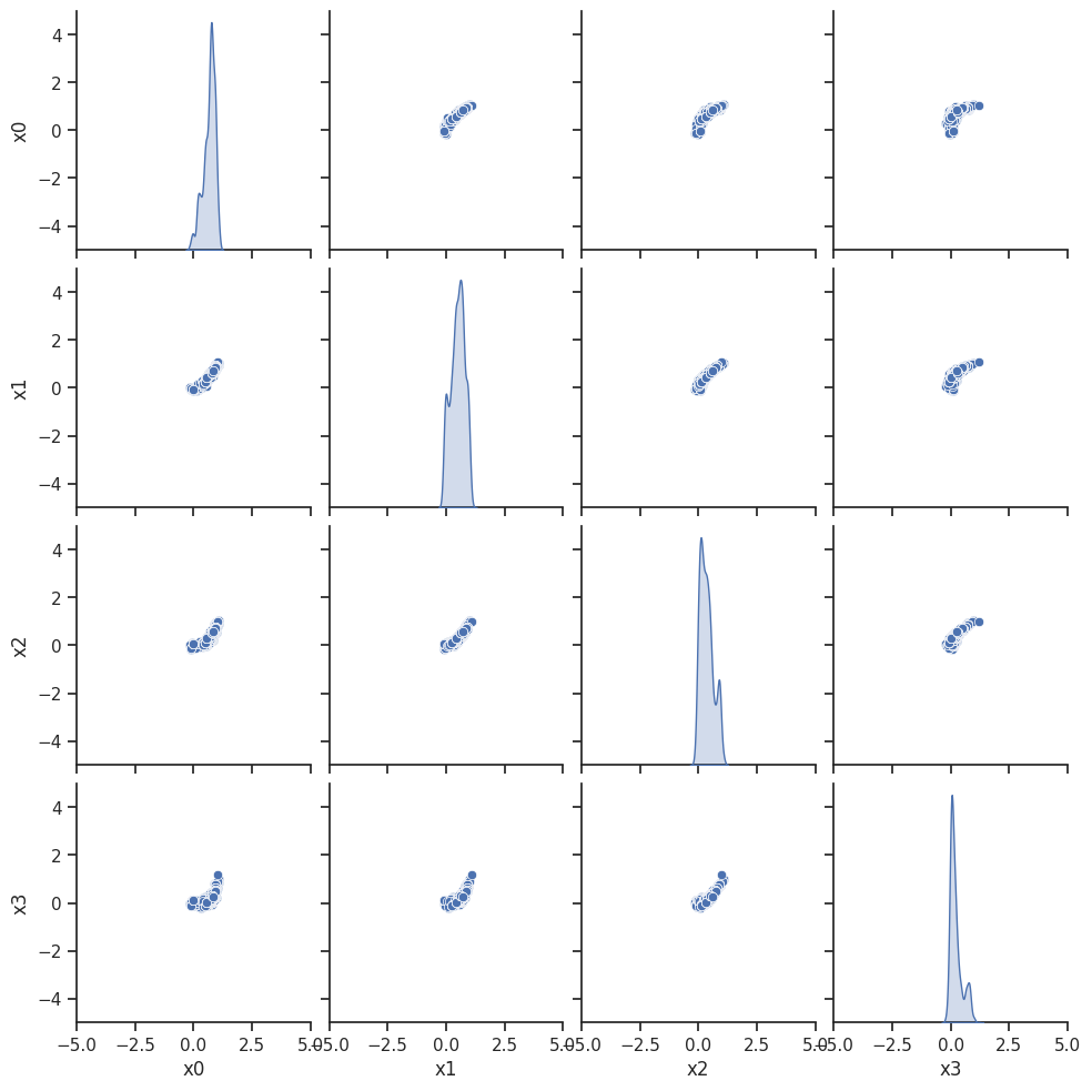
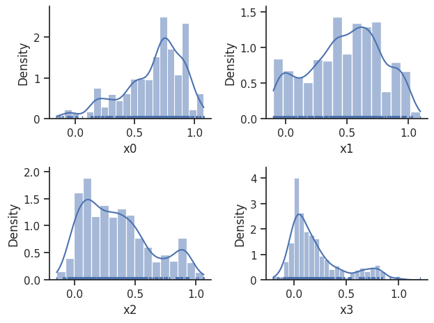
2-dim test problem: Rosenbrock banana
The adaptive parallel tempering sampler with chains running adaptive Metropolis samplers is also able to sample from more challenging posterior distributions. To illustrates this shortly, we use the Rosenbrock function.
[36]:
import scipy.optimize as so

import pypesto

# first type of objective
objective = pypesto.Objective(fun=so.rosen)

dim_full = 4
lb = -5 * np.ones((dim_full, 1))
ub = 5 * np.ones((dim_full, 1))

problem = pypesto.Problem(objective=objective, lb=lb, ub=ub)
[37]:
sampler = sample.AdaptiveParallelTemperingSampler(
    internal_sampler=sample.AdaptiveMetropolisSampler(), n_chains=10
)
result = sample.sample(
    problem, 2e3, sampler, x0=np.zeros(dim_full), filename=None
)
Initializing betas with "near-exponential decay".
Initializing parallel chains with a combination of the starting point and prior samples with weight: 0.9.
Elapsed time: 3.9791187200000024
[38]:
sample.geweke_test(result)
ax = visualize.sampling_scatter(result)
ax = visualize.sampling_1d_marginals(result)
Geweke burn-in index: 800