Parameter estimation using non-linear semi-quantitative data
In this notebook we illustrate how to use non-linear semi-quantitatiave data for parameter optimization in pyPESTO. An example model is provided in pypesto/doc/example/example_censored.
Some measurement techniques do not ensure a linear relationship between the abundance of the biochemical quantities of interest and the measured output . Well-known examples include fluorescence microscopy data like F ̈orster resonance energy transfer (FRET) data (Birtwistle et al. [2011]), optical density (OD) measurement (Stevenson et al. [2016]) and imaging data for certain stainings (Pargett et al. [2014]).
Assuming a Gaussian distributed additive noise model, a non-linear semi-quantitative type observable has the following relationship between the biochemical quantities of intereset \((y_k = h(x(t_k, \theta), \theta))_{k=1}^{n_t}\) and the measured quantities \((\widetilde{z}_k)_{k=1}^N\)
Where:
\(\{y_k\}_{k=1}^N\) is the model output at timepoints \(\{t_k\}_{k=1}^N\),
\(\{\varepsilon_k\}_{k=1}^N\) is the normally distributed measurement noise,
and \(\theta\) is the vector of model (unknown) mechanistic model parameters.
In pyPESTO, we have implemented an alogorithm which constructs and optimizes a spline approximation \(s(y, \xi)\) (to be exact, a piecewise linear function) of the non-linear monotone function \(g(y_k)\).
Using this spline appoximation of the function \(g\) we can then obtain spline-mapped simulations \(\{z_k = s(y_k, \xi)\}_{k=1}^N\) that are comparable to the measured quantities. Thus, we can define a negative log-likelihood objective function and optimize it to obtain maximum likelihood estimates. For better efficiency, the objective function is optimized hierarchically
The dynamical parameters \(\theta\) are optimized in the outer hierarchical loop,
The spline parameters \(\xi\) are optimized in the inner loop for each iteration of the outer one.
In the following we will demonstrate how to use the spline approximation approach for integration of nonlinear-monotone data.
Problem specification & importing model from the petab_problem
[1]:
import matplotlib.pyplot as plt
import numpy as np
import petab

import pypesto
import pypesto.logging
import pypesto.optimize as optimize
import pypesto.petab
from pypesto.C import LIN, InnerParameterType
from pypesto.hierarchical.semiquantitative import (
    SemiquantInnerSolver,
    SemiquantProblem,
)
from pypesto.hierarchical.semiquantitative.parameter import (
    SplineInnerParameter,
)
from pypesto.visualize import (
    plot_splines_from_inner_result,
    visualize_estimated_observable_mapping,
)
from pypesto.visualize.model_fit import visualize_optimized_model_fit
As the spline approach is implemented in the hierarchical manner, it requires us to specify hierarchical=True to the petab importer:
[2]:
petab_folder = "./example_semiquantitative/"
yaml_file = "example_semiquantitative.yaml"

petab_problem = petab.Problem.from_yaml(petab_folder + yaml_file)

importer = pypesto.petab.PetabImporter(petab_problem, hierarchical=True)
Visualization table not available. Skipping.
To estimate the noise parameters of the nonlinear-monotone observables, those noise parameters in the parameter.tsv file have to have column entries estimate with value 1 and column entry parameterType with value sigma, as in case of using relative (scaling+offset) data:
[3]:
import pandas as pd
from pandas import option_context

noise_parameter_file = "parameters_example_semiquantitative_noise.tsv"
# load the csv file
noise_parameter_df = pd.read_csv(petab_folder + noise_parameter_file, sep="\t")
with option_context("display.max_colwidth", 400):
    display(noise_parameter_df)
| parameterId | parameterName | parameterScale | lowerBound | upperBound | nominalValue | estimate | parameterType | |
|---|---|---|---|---|---|---|---|---|
| 0 | K1 | K1 | lin | -5.00000 | 5.0 | 0.04 | 0 | NaN |
| 1 | K2 | K2 | lin | -5.00000 | 5.0 | 20.00 | 0 | NaN |
| 2 | K3 | K3 | log10 | 0.10000 | 100000.0 | 4000.00 | 1 | NaN |
| 3 | K5 | K5 | log10 | 0.00001 | 100000.0 | 0.10 | 1 | NaN |
| 4 | sd_Activity | \sigma_{activity} | lin | 0.00000 | inf | 1.00 | 1 | sigma |
| 5 | sd_Ybar | \sigma_{ybar} | lin | 0.00000 | inf | 1.00 | 1 | sigma |
The only difference in the PEtab formulation is in the measurementType column of the measurement file. The non-linear (monotone) semi-quantitative measurements have to be specified file by adding semiquantitative in this column.
[4]:
with option_context("display.max_colwidth", 400):
    display(petab_problem.measurement_df)
| observableId | preequilibrationConditionId | simulationConditionId | measurement | time | observableParameters | noiseParameters | observableTransformation | noiseDistribution | measurementType | |
|---|---|---|---|---|---|---|---|---|---|---|
| 0 | Activity | NaN | Inhibitor_0 | 7.682403 | 5 | NaN | 1 | lin | normal | semiquantitative |
| 1 | Activity | NaN | Inhibitor_3 | 7.876107 | 5 | NaN | 1 | lin | normal | semiquantitative |
| 2 | Activity | NaN | Inhibitor_10 | 8.314587 | 5 | NaN | 1 | lin | normal | semiquantitative |
| 3 | Activity | NaN | Inhibitor_25 | 9.130915 | 5 | NaN | 1 | lin | normal | semiquantitative |
| 4 | Activity | NaN | Inhibitor_35 | 8.078494 | 5 | NaN | 1 | lin | normal | semiquantitative |
| 5 | Activity | NaN | Inhibitor_50 | 5.452116 | 5 | NaN | 1 | lin | normal | semiquantitative |
| 6 | Activity | NaN | Inhibitor_75 | 2.698746 | 5 | NaN | 1 | lin | normal | semiquantitative |
| 7 | Activity | NaN | Inhibitor_100 | 1.673154 | 5 | NaN | 1 | lin | normal | semiquantitative |
| 8 | Activity | NaN | Inhibitor_300 | 0.392886 | 5 | NaN | 1 | lin | normal | semiquantitative |
| 9 | Ybar | NaN | Inhibitor_0 | 0.000000 | 5 | NaN | 1 | lin | normal | semiquantitative |
| 10 | Ybar | NaN | Inhibitor_3 | 0.744411 | 5 | NaN | 1 | lin | normal | semiquantitative |
| 11 | Ybar | NaN | Inhibitor_10 | 2.310524 | 5 | NaN | 1 | lin | normal | semiquantitative |
| 12 | Ybar | NaN | Inhibitor_25 | 4.238056 | 5 | NaN | 1 | lin | normal | semiquantitative |
| 13 | Ybar | NaN | Inhibitor_35 | 4.642859 | 5 | NaN | 1 | lin | normal | semiquantitative |
| 14 | Ybar | NaN | Inhibitor_50 | 4.832879 | 5 | NaN | 1 | lin | normal | semiquantitative |
| 15 | Ybar | NaN | Inhibitor_75 | 4.898684 | 5 | NaN | 1 | lin | normal | semiquantitative |
| 16 | Ybar | NaN | Inhibitor_100 | 4.913791 | 5 | NaN | 1 | lin | normal | semiquantitative |
| 17 | Ybar | NaN | Inhibitor_300 | 4.929008 | 5 | NaN | 1 | lin | normal | semiquantitative |
Note on inclusion of additional data types:
It is possible to include observables with different types of data to the same petab_problem. Refer to the notebooks on using relative data, ordinal data and censored data for details on integration of other data types. If the measurementType column is left empty for all measurements of an observable, the observable will be treated as quantitative.
Constructing the objective and pypesto problem
The spline approximation options that can be specified are the following
spline_ratio: float value, determines the number of spline knots asn_spline_pars=spline_ratio*n_datapointsmin_diff_factor: float value, determines the minimal difference between consecutive spline heights asmin_diff_factor*measurement_range/n_spline_pars. Set it to 0.0 to disable.regularize_spline: boolean value, determines whether the spline is regularized by a linear function. In most cases, this this option improves method convergence. The goal is to reduce false positive data non-linear splines by pushing them towards a linear line.regularization_factor: float value, determines the strength of the regularization. It is the \(\lambda\) factor in the objective function \(J(\theta, \xi) = -\log \mathcal{L}_{\mathcal{D}}(\theta, \xi) + \lambda R(\xi)\), where \(-\log \mathcal{L}_{\mathcal{D}}(\theta, \xi)\) is the negative log-likelihood and \(R(\xi)\) is the regularization.
The min_diff_factor is a multiplier of the minimal difference between spline heights. Positive values act as a penalty in the objective function for incorrect orderings; this penalty can improve convergence for most models. However, high min_diff_factor values will reduce the spline’s ability to approximate functions with flat regions accurately. This issue will be demonstrated in the last section.
Now when we construct the objective, it will construct all objects of the spline inner optimization for semi-quantitative data:
SemiquantInnerSolverSemiquantCalculatorSemiquantProblem
Specifically, the SemiquantInnerSolver and SemiquantProblem will be constructed with default settings of
spline_ratio= 1/2use_minimal_difference= 0.0regularize_spline= Falseregularization_factor= 0.0
[5]:
factory = importer.create_objective_creator()
objective = factory.create_objective(verbose=False)
2026-06-08 09:58:24.391 - amici.sim.sundials.petab.v1._parameter_mapping - DEBUG - PEtab mapping: ({}, {'K1': 'K1', 'K2': 'K2', 'K3': 'K3', 'K5': 'K5', 'init_I': 0.0, 'Dimerize_k2': 1.0, 'Dimerize_RI_k2': 1.0, 'Inhibit_k2': 1.0, 'Inhibit_RR_k2': 1.0, 'Inhibit_RIR_k2': 1.0, 'Dimerize_R_RI_k2': 1.0, 'noiseParameter1_Activity': 1, 'noiseParameter1_Ybar': 1}, {}, {'K1': 'lin', 'K2': 'lin', 'K3': 'log10', 'K5': 'log10', 'init_I': 'lin', 'Dimerize_k2': 'lin', 'Dimerize_RI_k2': 'lin', 'Inhibit_k2': 'lin', 'Inhibit_RR_k2': 'lin', 'Inhibit_RIR_k2': 'lin', 'Dimerize_R_RI_k2': 'lin', 'noiseParameter1_Activity': 'lin', 'noiseParameter1_Ybar': 'lin'})
2026-06-08 09:58:24.392 - amici.sim.sundials.petab.v1._parameter_mapping - DEBUG - Fixed parameters pre-equilibration: {}
2026-06-08 09:58:24.393 - amici.sim.sundials.petab.v1._parameter_mapping - DEBUG - Fixed parameters simulation: {'K1': 'K1', 'K2': 'K2', 'init_I': 0.0}
2026-06-08 09:58:24.394 - amici.sim.sundials.petab.v1._parameter_mapping - DEBUG - Variable parameters pre-equilibration: {}
2026-06-08 09:58:24.394 - amici.sim.sundials.petab.v1._parameter_mapping - DEBUG - Variable parameters simulation: {'K3': 'K3', 'K5': 'K5', 'Dimerize_k2': 1.0, 'Dimerize_RI_k2': 1.0, 'Inhibit_k2': 1.0, 'Inhibit_RR_k2': 1.0, 'Inhibit_RIR_k2': 1.0, 'Dimerize_R_RI_k2': 1.0, 'noiseParameter1_Activity': 1, 'noiseParameter1_Ybar': 1}
2026-06-08 09:58:24.395 - amici.sim.sundials.petab.v1._parameter_mapping - DEBUG - Merged: {'K3': 'K3', 'K5': 'K5', 'Dimerize_k2': 1.0, 'Dimerize_RI_k2': 1.0, 'Inhibit_k2': 1.0, 'Inhibit_RR_k2': 1.0, 'Inhibit_RIR_k2': 1.0, 'Dimerize_R_RI_k2': 1.0, 'noiseParameter1_Activity': 1, 'noiseParameter1_Ybar': 1}
2026-06-08 09:58:24.396 - amici.sim.sundials.petab.v1._parameter_mapping - DEBUG - PEtab mapping: ({}, {'K1': 'K1', 'K2': 'K2', 'K3': 'K3', 'K5': 'K5', 'init_I': 10.0, 'Dimerize_k2': 1.0, 'Dimerize_RI_k2': 1.0, 'Inhibit_k2': 1.0, 'Inhibit_RR_k2': 1.0, 'Inhibit_RIR_k2': 1.0, 'Dimerize_R_RI_k2': 1.0, 'noiseParameter1_Activity': 1, 'noiseParameter1_Ybar': 1}, {}, {'K1': 'lin', 'K2': 'lin', 'K3': 'log10', 'K5': 'log10', 'init_I': 'lin', 'Dimerize_k2': 'lin', 'Dimerize_RI_k2': 'lin', 'Inhibit_k2': 'lin', 'Inhibit_RR_k2': 'lin', 'Inhibit_RIR_k2': 'lin', 'Dimerize_R_RI_k2': 'lin', 'noiseParameter1_Activity': 'lin', 'noiseParameter1_Ybar': 'lin'})
2026-06-08 09:58:24.397 - amici.sim.sundials.petab.v1._parameter_mapping - DEBUG - Fixed parameters pre-equilibration: {}
2026-06-08 09:58:24.398 - amici.sim.sundials.petab.v1._parameter_mapping - DEBUG - Fixed parameters simulation: {'K1': 'K1', 'K2': 'K2', 'init_I': 10.0}
2026-06-08 09:58:24.399 - amici.sim.sundials.petab.v1._parameter_mapping - DEBUG - Variable parameters pre-equilibration: {}
2026-06-08 09:58:24.400 - amici.sim.sundials.petab.v1._parameter_mapping - DEBUG - Variable parameters simulation: {'K3': 'K3', 'K5': 'K5', 'Dimerize_k2': 1.0, 'Dimerize_RI_k2': 1.0, 'Inhibit_k2': 1.0, 'Inhibit_RR_k2': 1.0, 'Inhibit_RIR_k2': 1.0, 'Dimerize_R_RI_k2': 1.0, 'noiseParameter1_Activity': 1, 'noiseParameter1_Ybar': 1}
2026-06-08 09:58:24.400 - amici.sim.sundials.petab.v1._parameter_mapping - DEBUG - Merged: {'K3': 'K3', 'K5': 'K5', 'Dimerize_k2': 1.0, 'Dimerize_RI_k2': 1.0, 'Inhibit_k2': 1.0, 'Inhibit_RR_k2': 1.0, 'Inhibit_RIR_k2': 1.0, 'Dimerize_R_RI_k2': 1.0, 'noiseParameter1_Activity': 1, 'noiseParameter1_Ybar': 1}
2026-06-08 09:58:24.401 - amici.sim.sundials.petab.v1._parameter_mapping - DEBUG - PEtab mapping: ({}, {'K1': 'K1', 'K2': 'K2', 'K3': 'K3', 'K5': 'K5', 'init_I': 100.0, 'Dimerize_k2': 1.0, 'Dimerize_RI_k2': 1.0, 'Inhibit_k2': 1.0, 'Inhibit_RR_k2': 1.0, 'Inhibit_RIR_k2': 1.0, 'Dimerize_R_RI_k2': 1.0, 'noiseParameter1_Activity': 1, 'noiseParameter1_Ybar': 1}, {}, {'K1': 'lin', 'K2': 'lin', 'K3': 'log10', 'K5': 'log10', 'init_I': 'lin', 'Dimerize_k2': 'lin', 'Dimerize_RI_k2': 'lin', 'Inhibit_k2': 'lin', 'Inhibit_RR_k2': 'lin', 'Inhibit_RIR_k2': 'lin', 'Dimerize_R_RI_k2': 'lin', 'noiseParameter1_Activity': 'lin', 'noiseParameter1_Ybar': 'lin'})
2026-06-08 09:58:24.401 - amici.sim.sundials.petab.v1._parameter_mapping - DEBUG - Fixed parameters pre-equilibration: {}
2026-06-08 09:58:24.402 - amici.sim.sundials.petab.v1._parameter_mapping - DEBUG - Fixed parameters simulation: {'K1': 'K1', 'K2': 'K2', 'init_I': 100.0}
2026-06-08 09:58:24.403 - amici.sim.sundials.petab.v1._parameter_mapping - DEBUG - Variable parameters pre-equilibration: {}
2026-06-08 09:58:24.404 - amici.sim.sundials.petab.v1._parameter_mapping - DEBUG - Variable parameters simulation: {'K3': 'K3', 'K5': 'K5', 'Dimerize_k2': 1.0, 'Dimerize_RI_k2': 1.0, 'Inhibit_k2': 1.0, 'Inhibit_RR_k2': 1.0, 'Inhibit_RIR_k2': 1.0, 'Dimerize_R_RI_k2': 1.0, 'noiseParameter1_Activity': 1, 'noiseParameter1_Ybar': 1}
2026-06-08 09:58:24.404 - amici.sim.sundials.petab.v1._parameter_mapping - DEBUG - Merged: {'K3': 'K3', 'K5': 'K5', 'Dimerize_k2': 1.0, 'Dimerize_RI_k2': 1.0, 'Inhibit_k2': 1.0, 'Inhibit_RR_k2': 1.0, 'Inhibit_RIR_k2': 1.0, 'Dimerize_R_RI_k2': 1.0, 'noiseParameter1_Activity': 1, 'noiseParameter1_Ybar': 1}
2026-06-08 09:58:24.405 - amici.sim.sundials.petab.v1._parameter_mapping - DEBUG - PEtab mapping: ({}, {'K1': 'K1', 'K2': 'K2', 'K3': 'K3', 'K5': 'K5', 'init_I': 25.0, 'Dimerize_k2': 1.0, 'Dimerize_RI_k2': 1.0, 'Inhibit_k2': 1.0, 'Inhibit_RR_k2': 1.0, 'Inhibit_RIR_k2': 1.0, 'Dimerize_R_RI_k2': 1.0, 'noiseParameter1_Activity': 1, 'noiseParameter1_Ybar': 1}, {}, {'K1': 'lin', 'K2': 'lin', 'K3': 'log10', 'K5': 'log10', 'init_I': 'lin', 'Dimerize_k2': 'lin', 'Dimerize_RI_k2': 'lin', 'Inhibit_k2': 'lin', 'Inhibit_RR_k2': 'lin', 'Inhibit_RIR_k2': 'lin', 'Dimerize_R_RI_k2': 'lin', 'noiseParameter1_Activity': 'lin', 'noiseParameter1_Ybar': 'lin'})
2026-06-08 09:58:24.406 - amici.sim.sundials.petab.v1._parameter_mapping - DEBUG - Fixed parameters pre-equilibration: {}
2026-06-08 09:58:24.406 - amici.sim.sundials.petab.v1._parameter_mapping - DEBUG - Fixed parameters simulation: {'K1': 'K1', 'K2': 'K2', 'init_I': 25.0}
2026-06-08 09:58:24.407 - amici.sim.sundials.petab.v1._parameter_mapping - DEBUG - Variable parameters pre-equilibration: {}
2026-06-08 09:58:24.408 - amici.sim.sundials.petab.v1._parameter_mapping - DEBUG - Variable parameters simulation: {'K3': 'K3', 'K5': 'K5', 'Dimerize_k2': 1.0, 'Dimerize_RI_k2': 1.0, 'Inhibit_k2': 1.0, 'Inhibit_RR_k2': 1.0, 'Inhibit_RIR_k2': 1.0, 'Dimerize_R_RI_k2': 1.0, 'noiseParameter1_Activity': 1, 'noiseParameter1_Ybar': 1}
2026-06-08 09:58:24.408 - amici.sim.sundials.petab.v1._parameter_mapping - DEBUG - Merged: {'K3': 'K3', 'K5': 'K5', 'Dimerize_k2': 1.0, 'Dimerize_RI_k2': 1.0, 'Inhibit_k2': 1.0, 'Inhibit_RR_k2': 1.0, 'Inhibit_RIR_k2': 1.0, 'Dimerize_R_RI_k2': 1.0, 'noiseParameter1_Activity': 1, 'noiseParameter1_Ybar': 1}
2026-06-08 09:58:24.409 - amici.sim.sundials.petab.v1._parameter_mapping - DEBUG - PEtab mapping: ({}, {'K1': 'K1', 'K2': 'K2', 'K3': 'K3', 'K5': 'K5', 'init_I': 3.0, 'Dimerize_k2': 1.0, 'Dimerize_RI_k2': 1.0, 'Inhibit_k2': 1.0, 'Inhibit_RR_k2': 1.0, 'Inhibit_RIR_k2': 1.0, 'Dimerize_R_RI_k2': 1.0, 'noiseParameter1_Activity': 1, 'noiseParameter1_Ybar': 1}, {}, {'K1': 'lin', 'K2': 'lin', 'K3': 'log10', 'K5': 'log10', 'init_I': 'lin', 'Dimerize_k2': 'lin', 'Dimerize_RI_k2': 'lin', 'Inhibit_k2': 'lin', 'Inhibit_RR_k2': 'lin', 'Inhibit_RIR_k2': 'lin', 'Dimerize_R_RI_k2': 'lin', 'noiseParameter1_Activity': 'lin', 'noiseParameter1_Ybar': 'lin'})
2026-06-08 09:58:24.409 - amici.sim.sundials.petab.v1._parameter_mapping - DEBUG - Fixed parameters pre-equilibration: {}
2026-06-08 09:58:24.410 - amici.sim.sundials.petab.v1._parameter_mapping - DEBUG - Fixed parameters simulation: {'K1': 'K1', 'K2': 'K2', 'init_I': 3.0}
2026-06-08 09:58:24.410 - amici.sim.sundials.petab.v1._parameter_mapping - DEBUG - Variable parameters pre-equilibration: {}
2026-06-08 09:58:24.411 - amici.sim.sundials.petab.v1._parameter_mapping - DEBUG - Variable parameters simulation: {'K3': 'K3', 'K5': 'K5', 'Dimerize_k2': 1.0, 'Dimerize_RI_k2': 1.0, 'Inhibit_k2': 1.0, 'Inhibit_RR_k2': 1.0, 'Inhibit_RIR_k2': 1.0, 'Dimerize_R_RI_k2': 1.0, 'noiseParameter1_Activity': 1, 'noiseParameter1_Ybar': 1}
2026-06-08 09:58:24.411 - amici.sim.sundials.petab.v1._parameter_mapping - DEBUG - Merged: {'K3': 'K3', 'K5': 'K5', 'Dimerize_k2': 1.0, 'Dimerize_RI_k2': 1.0, 'Inhibit_k2': 1.0, 'Inhibit_RR_k2': 1.0, 'Inhibit_RIR_k2': 1.0, 'Dimerize_R_RI_k2': 1.0, 'noiseParameter1_Activity': 1, 'noiseParameter1_Ybar': 1}
2026-06-08 09:58:24.412 - amici.sim.sundials.petab.v1._parameter_mapping - DEBUG - PEtab mapping: ({}, {'K1': 'K1', 'K2': 'K2', 'K3': 'K3', 'K5': 'K5', 'init_I': 300.0, 'Dimerize_k2': 1.0, 'Dimerize_RI_k2': 1.0, 'Inhibit_k2': 1.0, 'Inhibit_RR_k2': 1.0, 'Inhibit_RIR_k2': 1.0, 'Dimerize_R_RI_k2': 1.0, 'noiseParameter1_Activity': 1, 'noiseParameter1_Ybar': 1}, {}, {'K1': 'lin', 'K2': 'lin', 'K3': 'log10', 'K5': 'log10', 'init_I': 'lin', 'Dimerize_k2': 'lin', 'Dimerize_RI_k2': 'lin', 'Inhibit_k2': 'lin', 'Inhibit_RR_k2': 'lin', 'Inhibit_RIR_k2': 'lin', 'Dimerize_R_RI_k2': 'lin', 'noiseParameter1_Activity': 'lin', 'noiseParameter1_Ybar': 'lin'})
2026-06-08 09:58:24.413 - amici.sim.sundials.petab.v1._parameter_mapping - DEBUG - Fixed parameters pre-equilibration: {}
2026-06-08 09:58:24.414 - amici.sim.sundials.petab.v1._parameter_mapping - DEBUG - Fixed parameters simulation: {'K1': 'K1', 'K2': 'K2', 'init_I': 300.0}
2026-06-08 09:58:24.414 - amici.sim.sundials.petab.v1._parameter_mapping - DEBUG - Variable parameters pre-equilibration: {}
2026-06-08 09:58:24.415 - amici.sim.sundials.petab.v1._parameter_mapping - DEBUG - Variable parameters simulation: {'K3': 'K3', 'K5': 'K5', 'Dimerize_k2': 1.0, 'Dimerize_RI_k2': 1.0, 'Inhibit_k2': 1.0, 'Inhibit_RR_k2': 1.0, 'Inhibit_RIR_k2': 1.0, 'Dimerize_R_RI_k2': 1.0, 'noiseParameter1_Activity': 1, 'noiseParameter1_Ybar': 1}
2026-06-08 09:58:24.416 - amici.sim.sundials.petab.v1._parameter_mapping - DEBUG - Merged: {'K3': 'K3', 'K5': 'K5', 'Dimerize_k2': 1.0, 'Dimerize_RI_k2': 1.0, 'Inhibit_k2': 1.0, 'Inhibit_RR_k2': 1.0, 'Inhibit_RIR_k2': 1.0, 'Dimerize_R_RI_k2': 1.0, 'noiseParameter1_Activity': 1, 'noiseParameter1_Ybar': 1}
2026-06-08 09:58:24.416 - amici.sim.sundials.petab.v1._parameter_mapping - DEBUG - PEtab mapping: ({}, {'K1': 'K1', 'K2': 'K2', 'K3': 'K3', 'K5': 'K5', 'init_I': 35.0, 'Dimerize_k2': 1.0, 'Dimerize_RI_k2': 1.0, 'Inhibit_k2': 1.0, 'Inhibit_RR_k2': 1.0, 'Inhibit_RIR_k2': 1.0, 'Dimerize_R_RI_k2': 1.0, 'noiseParameter1_Activity': 1, 'noiseParameter1_Ybar': 1}, {}, {'K1': 'lin', 'K2': 'lin', 'K3': 'log10', 'K5': 'log10', 'init_I': 'lin', 'Dimerize_k2': 'lin', 'Dimerize_RI_k2': 'lin', 'Inhibit_k2': 'lin', 'Inhibit_RR_k2': 'lin', 'Inhibit_RIR_k2': 'lin', 'Dimerize_R_RI_k2': 'lin', 'noiseParameter1_Activity': 'lin', 'noiseParameter1_Ybar': 'lin'})
2026-06-08 09:58:24.417 - amici.sim.sundials.petab.v1._parameter_mapping - DEBUG - Fixed parameters pre-equilibration: {}
2026-06-08 09:58:24.417 - amici.sim.sundials.petab.v1._parameter_mapping - DEBUG - Fixed parameters simulation: {'K1': 'K1', 'K2': 'K2', 'init_I': 35.0}
2026-06-08 09:58:24.418 - amici.sim.sundials.petab.v1._parameter_mapping - DEBUG - Variable parameters pre-equilibration: {}
2026-06-08 09:58:24.418 - amici.sim.sundials.petab.v1._parameter_mapping - DEBUG - Variable parameters simulation: {'K3': 'K3', 'K5': 'K5', 'Dimerize_k2': 1.0, 'Dimerize_RI_k2': 1.0, 'Inhibit_k2': 1.0, 'Inhibit_RR_k2': 1.0, 'Inhibit_RIR_k2': 1.0, 'Dimerize_R_RI_k2': 1.0, 'noiseParameter1_Activity': 1, 'noiseParameter1_Ybar': 1}
2026-06-08 09:58:24.419 - amici.sim.sundials.petab.v1._parameter_mapping - DEBUG - Merged: {'K3': 'K3', 'K5': 'K5', 'Dimerize_k2': 1.0, 'Dimerize_RI_k2': 1.0, 'Inhibit_k2': 1.0, 'Inhibit_RR_k2': 1.0, 'Inhibit_RIR_k2': 1.0, 'Dimerize_R_RI_k2': 1.0, 'noiseParameter1_Activity': 1, 'noiseParameter1_Ybar': 1}
2026-06-08 09:58:24.420 - amici.sim.sundials.petab.v1._parameter_mapping - DEBUG - PEtab mapping: ({}, {'K1': 'K1', 'K2': 'K2', 'K3': 'K3', 'K5': 'K5', 'init_I': 50.0, 'Dimerize_k2': 1.0, 'Dimerize_RI_k2': 1.0, 'Inhibit_k2': 1.0, 'Inhibit_RR_k2': 1.0, 'Inhibit_RIR_k2': 1.0, 'Dimerize_R_RI_k2': 1.0, 'noiseParameter1_Activity': 1, 'noiseParameter1_Ybar': 1}, {}, {'K1': 'lin', 'K2': 'lin', 'K3': 'log10', 'K5': 'log10', 'init_I': 'lin', 'Dimerize_k2': 'lin', 'Dimerize_RI_k2': 'lin', 'Inhibit_k2': 'lin', 'Inhibit_RR_k2': 'lin', 'Inhibit_RIR_k2': 'lin', 'Dimerize_R_RI_k2': 'lin', 'noiseParameter1_Activity': 'lin', 'noiseParameter1_Ybar': 'lin'})
2026-06-08 09:58:24.422 - amici.sim.sundials.petab.v1._parameter_mapping - DEBUG - Fixed parameters pre-equilibration: {}
2026-06-08 09:58:24.422 - amici.sim.sundials.petab.v1._parameter_mapping - DEBUG - Fixed parameters simulation: {'K1': 'K1', 'K2': 'K2', 'init_I': 50.0}
2026-06-08 09:58:24.423 - amici.sim.sundials.petab.v1._parameter_mapping - DEBUG - Variable parameters pre-equilibration: {}
2026-06-08 09:58:24.423 - amici.sim.sundials.petab.v1._parameter_mapping - DEBUG - Variable parameters simulation: {'K3': 'K3', 'K5': 'K5', 'Dimerize_k2': 1.0, 'Dimerize_RI_k2': 1.0, 'Inhibit_k2': 1.0, 'Inhibit_RR_k2': 1.0, 'Inhibit_RIR_k2': 1.0, 'Dimerize_R_RI_k2': 1.0, 'noiseParameter1_Activity': 1, 'noiseParameter1_Ybar': 1}
2026-06-08 09:58:24.424 - amici.sim.sundials.petab.v1._parameter_mapping - DEBUG - Merged: {'K3': 'K3', 'K5': 'K5', 'Dimerize_k2': 1.0, 'Dimerize_RI_k2': 1.0, 'Inhibit_k2': 1.0, 'Inhibit_RR_k2': 1.0, 'Inhibit_RIR_k2': 1.0, 'Dimerize_R_RI_k2': 1.0, 'noiseParameter1_Activity': 1, 'noiseParameter1_Ybar': 1}
2026-06-08 09:58:24.425 - amici.sim.sundials.petab.v1._parameter_mapping - DEBUG - PEtab mapping: ({}, {'K1': 'K1', 'K2': 'K2', 'K3': 'K3', 'K5': 'K5', 'init_I': 75.0, 'Dimerize_k2': 1.0, 'Dimerize_RI_k2': 1.0, 'Inhibit_k2': 1.0, 'Inhibit_RR_k2': 1.0, 'Inhibit_RIR_k2': 1.0, 'Dimerize_R_RI_k2': 1.0, 'noiseParameter1_Activity': 1, 'noiseParameter1_Ybar': 1}, {}, {'K1': 'lin', 'K2': 'lin', 'K3': 'log10', 'K5': 'log10', 'init_I': 'lin', 'Dimerize_k2': 'lin', 'Dimerize_RI_k2': 'lin', 'Inhibit_k2': 'lin', 'Inhibit_RR_k2': 'lin', 'Inhibit_RIR_k2': 'lin', 'Dimerize_R_RI_k2': 'lin', 'noiseParameter1_Activity': 'lin', 'noiseParameter1_Ybar': 'lin'})
2026-06-08 09:58:24.425 - amici.sim.sundials.petab.v1._parameter_mapping - DEBUG - Fixed parameters pre-equilibration: {}
2026-06-08 09:58:24.426 - amici.sim.sundials.petab.v1._parameter_mapping - DEBUG - Fixed parameters simulation: {'K1': 'K1', 'K2': 'K2', 'init_I': 75.0}
2026-06-08 09:58:24.426 - amici.sim.sundials.petab.v1._parameter_mapping - DEBUG - Variable parameters pre-equilibration: {}
2026-06-08 09:58:24.427 - amici.sim.sundials.petab.v1._parameter_mapping - DEBUG - Variable parameters simulation: {'K3': 'K3', 'K5': 'K5', 'Dimerize_k2': 1.0, 'Dimerize_RI_k2': 1.0, 'Inhibit_k2': 1.0, 'Inhibit_RR_k2': 1.0, 'Inhibit_RIR_k2': 1.0, 'Dimerize_R_RI_k2': 1.0, 'noiseParameter1_Activity': 1, 'noiseParameter1_Ybar': 1}
2026-06-08 09:58:24.427 - amici.sim.sundials.petab.v1._parameter_mapping - DEBUG - Merged: {'K3': 'K3', 'K5': 'K5', 'Dimerize_k2': 1.0, 'Dimerize_RI_k2': 1.0, 'Inhibit_k2': 1.0, 'Inhibit_RR_k2': 1.0, 'Inhibit_RIR_k2': 1.0, 'Dimerize_R_RI_k2': 1.0, 'noiseParameter1_Activity': 1, 'noiseParameter1_Ybar': 1}
To give non-default options to the OptimalScalingInnerSolver and OptimalScalingProblem, one can pass them as arguments when constructing the objective:
[6]:
objective = factory.create_objective(
    inner_options={
        "spline_ratio": 1 / 2,
        "min_diff_factor": 1 / 2,
        "regularize_spline": True,
        "regularization_factor": 1e-1,
    },
    verbose=False,
)
2026-06-08 09:58:24.540 - amici.sim.sundials.petab.v1._parameter_mapping - DEBUG - PEtab mapping: ({}, {'K1': 'K1', 'K2': 'K2', 'K3': 'K3', 'K5': 'K5', 'init_I': 0.0, 'Dimerize_k2': 1.0, 'Dimerize_RI_k2': 1.0, 'Inhibit_k2': 1.0, 'Inhibit_RR_k2': 1.0, 'Inhibit_RIR_k2': 1.0, 'Dimerize_R_RI_k2': 1.0, 'noiseParameter1_Activity': 1, 'noiseParameter1_Ybar': 1}, {}, {'K1': 'lin', 'K2': 'lin', 'K3': 'log10', 'K5': 'log10', 'init_I': 'lin', 'Dimerize_k2': 'lin', 'Dimerize_RI_k2': 'lin', 'Inhibit_k2': 'lin', 'Inhibit_RR_k2': 'lin', 'Inhibit_RIR_k2': 'lin', 'Dimerize_R_RI_k2': 'lin', 'noiseParameter1_Activity': 'lin', 'noiseParameter1_Ybar': 'lin'})
2026-06-08 09:58:24.541 - amici.sim.sundials.petab.v1._parameter_mapping - DEBUG - Fixed parameters pre-equilibration: {}
2026-06-08 09:58:24.542 - amici.sim.sundials.petab.v1._parameter_mapping - DEBUG - Fixed parameters simulation: {'K1': 'K1', 'K2': 'K2', 'init_I': 0.0}
2026-06-08 09:58:24.543 - amici.sim.sundials.petab.v1._parameter_mapping - DEBUG - Variable parameters pre-equilibration: {}
2026-06-08 09:58:24.544 - amici.sim.sundials.petab.v1._parameter_mapping - DEBUG - Variable parameters simulation: {'K3': 'K3', 'K5': 'K5', 'Dimerize_k2': 1.0, 'Dimerize_RI_k2': 1.0, 'Inhibit_k2': 1.0, 'Inhibit_RR_k2': 1.0, 'Inhibit_RIR_k2': 1.0, 'Dimerize_R_RI_k2': 1.0, 'noiseParameter1_Activity': 1, 'noiseParameter1_Ybar': 1}
2026-06-08 09:58:24.545 - amici.sim.sundials.petab.v1._parameter_mapping - DEBUG - Merged: {'K3': 'K3', 'K5': 'K5', 'Dimerize_k2': 1.0, 'Dimerize_RI_k2': 1.0, 'Inhibit_k2': 1.0, 'Inhibit_RR_k2': 1.0, 'Inhibit_RIR_k2': 1.0, 'Dimerize_R_RI_k2': 1.0, 'noiseParameter1_Activity': 1, 'noiseParameter1_Ybar': 1}
2026-06-08 09:58:24.546 - amici.sim.sundials.petab.v1._parameter_mapping - DEBUG - PEtab mapping: ({}, {'K1': 'K1', 'K2': 'K2', 'K3': 'K3', 'K5': 'K5', 'init_I': 10.0, 'Dimerize_k2': 1.0, 'Dimerize_RI_k2': 1.0, 'Inhibit_k2': 1.0, 'Inhibit_RR_k2': 1.0, 'Inhibit_RIR_k2': 1.0, 'Dimerize_R_RI_k2': 1.0, 'noiseParameter1_Activity': 1, 'noiseParameter1_Ybar': 1}, {}, {'K1': 'lin', 'K2': 'lin', 'K3': 'log10', 'K5': 'log10', 'init_I': 'lin', 'Dimerize_k2': 'lin', 'Dimerize_RI_k2': 'lin', 'Inhibit_k2': 'lin', 'Inhibit_RR_k2': 'lin', 'Inhibit_RIR_k2': 'lin', 'Dimerize_R_RI_k2': 'lin', 'noiseParameter1_Activity': 'lin', 'noiseParameter1_Ybar': 'lin'})
2026-06-08 09:58:24.547 - amici.sim.sundials.petab.v1._parameter_mapping - DEBUG - Fixed parameters pre-equilibration: {}
2026-06-08 09:58:24.548 - amici.sim.sundials.petab.v1._parameter_mapping - DEBUG - Fixed parameters simulation: {'K1': 'K1', 'K2': 'K2', 'init_I': 10.0}
2026-06-08 09:58:24.548 - amici.sim.sundials.petab.v1._parameter_mapping - DEBUG - Variable parameters pre-equilibration: {}
2026-06-08 09:58:24.548 - amici.sim.sundials.petab.v1._parameter_mapping - DEBUG - Variable parameters simulation: {'K3': 'K3', 'K5': 'K5', 'Dimerize_k2': 1.0, 'Dimerize_RI_k2': 1.0, 'Inhibit_k2': 1.0, 'Inhibit_RR_k2': 1.0, 'Inhibit_RIR_k2': 1.0, 'Dimerize_R_RI_k2': 1.0, 'noiseParameter1_Activity': 1, 'noiseParameter1_Ybar': 1}
2026-06-08 09:58:24.549 - amici.sim.sundials.petab.v1._parameter_mapping - DEBUG - Merged: {'K3': 'K3', 'K5': 'K5', 'Dimerize_k2': 1.0, 'Dimerize_RI_k2': 1.0, 'Inhibit_k2': 1.0, 'Inhibit_RR_k2': 1.0, 'Inhibit_RIR_k2': 1.0, 'Dimerize_R_RI_k2': 1.0, 'noiseParameter1_Activity': 1, 'noiseParameter1_Ybar': 1}
2026-06-08 09:58:24.550 - amici.sim.sundials.petab.v1._parameter_mapping - DEBUG - PEtab mapping: ({}, {'K1': 'K1', 'K2': 'K2', 'K3': 'K3', 'K5': 'K5', 'init_I': 100.0, 'Dimerize_k2': 1.0, 'Dimerize_RI_k2': 1.0, 'Inhibit_k2': 1.0, 'Inhibit_RR_k2': 1.0, 'Inhibit_RIR_k2': 1.0, 'Dimerize_R_RI_k2': 1.0, 'noiseParameter1_Activity': 1, 'noiseParameter1_Ybar': 1}, {}, {'K1': 'lin', 'K2': 'lin', 'K3': 'log10', 'K5': 'log10', 'init_I': 'lin', 'Dimerize_k2': 'lin', 'Dimerize_RI_k2': 'lin', 'Inhibit_k2': 'lin', 'Inhibit_RR_k2': 'lin', 'Inhibit_RIR_k2': 'lin', 'Dimerize_R_RI_k2': 'lin', 'noiseParameter1_Activity': 'lin', 'noiseParameter1_Ybar': 'lin'})
2026-06-08 09:58:24.550 - amici.sim.sundials.petab.v1._parameter_mapping - DEBUG - Fixed parameters pre-equilibration: {}
2026-06-08 09:58:24.551 - amici.sim.sundials.petab.v1._parameter_mapping - DEBUG - Fixed parameters simulation: {'K1': 'K1', 'K2': 'K2', 'init_I': 100.0}
2026-06-08 09:58:24.551 - amici.sim.sundials.petab.v1._parameter_mapping - DEBUG - Variable parameters pre-equilibration: {}
2026-06-08 09:58:24.552 - amici.sim.sundials.petab.v1._parameter_mapping - DEBUG - Variable parameters simulation: {'K3': 'K3', 'K5': 'K5', 'Dimerize_k2': 1.0, 'Dimerize_RI_k2': 1.0, 'Inhibit_k2': 1.0, 'Inhibit_RR_k2': 1.0, 'Inhibit_RIR_k2': 1.0, 'Dimerize_R_RI_k2': 1.0, 'noiseParameter1_Activity': 1, 'noiseParameter1_Ybar': 1}
2026-06-08 09:58:24.554 - amici.sim.sundials.petab.v1._parameter_mapping - DEBUG - Merged: {'K3': 'K3', 'K5': 'K5', 'Dimerize_k2': 1.0, 'Dimerize_RI_k2': 1.0, 'Inhibit_k2': 1.0, 'Inhibit_RR_k2': 1.0, 'Inhibit_RIR_k2': 1.0, 'Dimerize_R_RI_k2': 1.0, 'noiseParameter1_Activity': 1, 'noiseParameter1_Ybar': 1}
2026-06-08 09:58:24.554 - amici.sim.sundials.petab.v1._parameter_mapping - DEBUG - PEtab mapping: ({}, {'K1': 'K1', 'K2': 'K2', 'K3': 'K3', 'K5': 'K5', 'init_I': 25.0, 'Dimerize_k2': 1.0, 'Dimerize_RI_k2': 1.0, 'Inhibit_k2': 1.0, 'Inhibit_RR_k2': 1.0, 'Inhibit_RIR_k2': 1.0, 'Dimerize_R_RI_k2': 1.0, 'noiseParameter1_Activity': 1, 'noiseParameter1_Ybar': 1}, {}, {'K1': 'lin', 'K2': 'lin', 'K3': 'log10', 'K5': 'log10', 'init_I': 'lin', 'Dimerize_k2': 'lin', 'Dimerize_RI_k2': 'lin', 'Inhibit_k2': 'lin', 'Inhibit_RR_k2': 'lin', 'Inhibit_RIR_k2': 'lin', 'Dimerize_R_RI_k2': 'lin', 'noiseParameter1_Activity': 'lin', 'noiseParameter1_Ybar': 'lin'})
2026-06-08 09:58:24.555 - amici.sim.sundials.petab.v1._parameter_mapping - DEBUG - Fixed parameters pre-equilibration: {}
2026-06-08 09:58:24.555 - amici.sim.sundials.petab.v1._parameter_mapping - DEBUG - Fixed parameters simulation: {'K1': 'K1', 'K2': 'K2', 'init_I': 25.0}
2026-06-08 09:58:24.556 - amici.sim.sundials.petab.v1._parameter_mapping - DEBUG - Variable parameters pre-equilibration: {}
2026-06-08 09:58:24.556 - amici.sim.sundials.petab.v1._parameter_mapping - DEBUG - Variable parameters simulation: {'K3': 'K3', 'K5': 'K5', 'Dimerize_k2': 1.0, 'Dimerize_RI_k2': 1.0, 'Inhibit_k2': 1.0, 'Inhibit_RR_k2': 1.0, 'Inhibit_RIR_k2': 1.0, 'Dimerize_R_RI_k2': 1.0, 'noiseParameter1_Activity': 1, 'noiseParameter1_Ybar': 1}
2026-06-08 09:58:24.557 - amici.sim.sundials.petab.v1._parameter_mapping - DEBUG - Merged: {'K3': 'K3', 'K5': 'K5', 'Dimerize_k2': 1.0, 'Dimerize_RI_k2': 1.0, 'Inhibit_k2': 1.0, 'Inhibit_RR_k2': 1.0, 'Inhibit_RIR_k2': 1.0, 'Dimerize_R_RI_k2': 1.0, 'noiseParameter1_Activity': 1, 'noiseParameter1_Ybar': 1}
2026-06-08 09:58:24.557 - amici.sim.sundials.petab.v1._parameter_mapping - DEBUG - PEtab mapping: ({}, {'K1': 'K1', 'K2': 'K2', 'K3': 'K3', 'K5': 'K5', 'init_I': 3.0, 'Dimerize_k2': 1.0, 'Dimerize_RI_k2': 1.0, 'Inhibit_k2': 1.0, 'Inhibit_RR_k2': 1.0, 'Inhibit_RIR_k2': 1.0, 'Dimerize_R_RI_k2': 1.0, 'noiseParameter1_Activity': 1, 'noiseParameter1_Ybar': 1}, {}, {'K1': 'lin', 'K2': 'lin', 'K3': 'log10', 'K5': 'log10', 'init_I': 'lin', 'Dimerize_k2': 'lin', 'Dimerize_RI_k2': 'lin', 'Inhibit_k2': 'lin', 'Inhibit_RR_k2': 'lin', 'Inhibit_RIR_k2': 'lin', 'Dimerize_R_RI_k2': 'lin', 'noiseParameter1_Activity': 'lin', 'noiseParameter1_Ybar': 'lin'})
2026-06-08 09:58:24.558 - amici.sim.sundials.petab.v1._parameter_mapping - DEBUG - Fixed parameters pre-equilibration: {}
2026-06-08 09:58:24.559 - amici.sim.sundials.petab.v1._parameter_mapping - DEBUG - Fixed parameters simulation: {'K1': 'K1', 'K2': 'K2', 'init_I': 3.0}
2026-06-08 09:58:24.559 - amici.sim.sundials.petab.v1._parameter_mapping - DEBUG - Variable parameters pre-equilibration: {}
2026-06-08 09:58:24.560 - amici.sim.sundials.petab.v1._parameter_mapping - DEBUG - Variable parameters simulation: {'K3': 'K3', 'K5': 'K5', 'Dimerize_k2': 1.0, 'Dimerize_RI_k2': 1.0, 'Inhibit_k2': 1.0, 'Inhibit_RR_k2': 1.0, 'Inhibit_RIR_k2': 1.0, 'Dimerize_R_RI_k2': 1.0, 'noiseParameter1_Activity': 1, 'noiseParameter1_Ybar': 1}
2026-06-08 09:58:24.560 - amici.sim.sundials.petab.v1._parameter_mapping - DEBUG - Merged: {'K3': 'K3', 'K5': 'K5', 'Dimerize_k2': 1.0, 'Dimerize_RI_k2': 1.0, 'Inhibit_k2': 1.0, 'Inhibit_RR_k2': 1.0, 'Inhibit_RIR_k2': 1.0, 'Dimerize_R_RI_k2': 1.0, 'noiseParameter1_Activity': 1, 'noiseParameter1_Ybar': 1}
2026-06-08 09:58:24.561 - amici.sim.sundials.petab.v1._parameter_mapping - DEBUG - PEtab mapping: ({}, {'K1': 'K1', 'K2': 'K2', 'K3': 'K3', 'K5': 'K5', 'init_I': 300.0, 'Dimerize_k2': 1.0, 'Dimerize_RI_k2': 1.0, 'Inhibit_k2': 1.0, 'Inhibit_RR_k2': 1.0, 'Inhibit_RIR_k2': 1.0, 'Dimerize_R_RI_k2': 1.0, 'noiseParameter1_Activity': 1, 'noiseParameter1_Ybar': 1}, {}, {'K1': 'lin', 'K2': 'lin', 'K3': 'log10', 'K5': 'log10', 'init_I': 'lin', 'Dimerize_k2': 'lin', 'Dimerize_RI_k2': 'lin', 'Inhibit_k2': 'lin', 'Inhibit_RR_k2': 'lin', 'Inhibit_RIR_k2': 'lin', 'Dimerize_R_RI_k2': 'lin', 'noiseParameter1_Activity': 'lin', 'noiseParameter1_Ybar': 'lin'})
2026-06-08 09:58:24.561 - amici.sim.sundials.petab.v1._parameter_mapping - DEBUG - Fixed parameters pre-equilibration: {}
2026-06-08 09:58:24.562 - amici.sim.sundials.petab.v1._parameter_mapping - DEBUG - Fixed parameters simulation: {'K1': 'K1', 'K2': 'K2', 'init_I': 300.0}
2026-06-08 09:58:24.562 - amici.sim.sundials.petab.v1._parameter_mapping - DEBUG - Variable parameters pre-equilibration: {}
2026-06-08 09:58:24.563 - amici.sim.sundials.petab.v1._parameter_mapping - DEBUG - Variable parameters simulation: {'K3': 'K3', 'K5': 'K5', 'Dimerize_k2': 1.0, 'Dimerize_RI_k2': 1.0, 'Inhibit_k2': 1.0, 'Inhibit_RR_k2': 1.0, 'Inhibit_RIR_k2': 1.0, 'Dimerize_R_RI_k2': 1.0, 'noiseParameter1_Activity': 1, 'noiseParameter1_Ybar': 1}
2026-06-08 09:58:24.564 - amici.sim.sundials.petab.v1._parameter_mapping - DEBUG - Merged: {'K3': 'K3', 'K5': 'K5', 'Dimerize_k2': 1.0, 'Dimerize_RI_k2': 1.0, 'Inhibit_k2': 1.0, 'Inhibit_RR_k2': 1.0, 'Inhibit_RIR_k2': 1.0, 'Dimerize_R_RI_k2': 1.0, 'noiseParameter1_Activity': 1, 'noiseParameter1_Ybar': 1}
2026-06-08 09:58:24.564 - amici.sim.sundials.petab.v1._parameter_mapping - DEBUG - PEtab mapping: ({}, {'K1': 'K1', 'K2': 'K2', 'K3': 'K3', 'K5': 'K5', 'init_I': 35.0, 'Dimerize_k2': 1.0, 'Dimerize_RI_k2': 1.0, 'Inhibit_k2': 1.0, 'Inhibit_RR_k2': 1.0, 'Inhibit_RIR_k2': 1.0, 'Dimerize_R_RI_k2': 1.0, 'noiseParameter1_Activity': 1, 'noiseParameter1_Ybar': 1}, {}, {'K1': 'lin', 'K2': 'lin', 'K3': 'log10', 'K5': 'log10', 'init_I': 'lin', 'Dimerize_k2': 'lin', 'Dimerize_RI_k2': 'lin', 'Inhibit_k2': 'lin', 'Inhibit_RR_k2': 'lin', 'Inhibit_RIR_k2': 'lin', 'Dimerize_R_RI_k2': 'lin', 'noiseParameter1_Activity': 'lin', 'noiseParameter1_Ybar': 'lin'})
2026-06-08 09:58:24.565 - amici.sim.sundials.petab.v1._parameter_mapping - DEBUG - Fixed parameters pre-equilibration: {}
2026-06-08 09:58:24.565 - amici.sim.sundials.petab.v1._parameter_mapping - DEBUG - Fixed parameters simulation: {'K1': 'K1', 'K2': 'K2', 'init_I': 35.0}
2026-06-08 09:58:24.566 - amici.sim.sundials.petab.v1._parameter_mapping - DEBUG - Variable parameters pre-equilibration: {}
2026-06-08 09:58:24.567 - amici.sim.sundials.petab.v1._parameter_mapping - DEBUG - Variable parameters simulation: {'K3': 'K3', 'K5': 'K5', 'Dimerize_k2': 1.0, 'Dimerize_RI_k2': 1.0, 'Inhibit_k2': 1.0, 'Inhibit_RR_k2': 1.0, 'Inhibit_RIR_k2': 1.0, 'Dimerize_R_RI_k2': 1.0, 'noiseParameter1_Activity': 1, 'noiseParameter1_Ybar': 1}
2026-06-08 09:58:24.567 - amici.sim.sundials.petab.v1._parameter_mapping - DEBUG - Merged: {'K3': 'K3', 'K5': 'K5', 'Dimerize_k2': 1.0, 'Dimerize_RI_k2': 1.0, 'Inhibit_k2': 1.0, 'Inhibit_RR_k2': 1.0, 'Inhibit_RIR_k2': 1.0, 'Dimerize_R_RI_k2': 1.0, 'noiseParameter1_Activity': 1, 'noiseParameter1_Ybar': 1}
2026-06-08 09:58:24.570 - amici.sim.sundials.petab.v1._parameter_mapping - DEBUG - PEtab mapping: ({}, {'K1': 'K1', 'K2': 'K2', 'K3': 'K3', 'K5': 'K5', 'init_I': 50.0, 'Dimerize_k2': 1.0, 'Dimerize_RI_k2': 1.0, 'Inhibit_k2': 1.0, 'Inhibit_RR_k2': 1.0, 'Inhibit_RIR_k2': 1.0, 'Dimerize_R_RI_k2': 1.0, 'noiseParameter1_Activity': 1, 'noiseParameter1_Ybar': 1}, {}, {'K1': 'lin', 'K2': 'lin', 'K3': 'log10', 'K5': 'log10', 'init_I': 'lin', 'Dimerize_k2': 'lin', 'Dimerize_RI_k2': 'lin', 'Inhibit_k2': 'lin', 'Inhibit_RR_k2': 'lin', 'Inhibit_RIR_k2': 'lin', 'Dimerize_R_RI_k2': 'lin', 'noiseParameter1_Activity': 'lin', 'noiseParameter1_Ybar': 'lin'})
2026-06-08 09:58:24.570 - amici.sim.sundials.petab.v1._parameter_mapping - DEBUG - Fixed parameters pre-equilibration: {}
2026-06-08 09:58:24.571 - amici.sim.sundials.petab.v1._parameter_mapping - DEBUG - Fixed parameters simulation: {'K1': 'K1', 'K2': 'K2', 'init_I': 50.0}
2026-06-08 09:58:24.571 - amici.sim.sundials.petab.v1._parameter_mapping - DEBUG - Variable parameters pre-equilibration: {}
2026-06-08 09:58:24.572 - amici.sim.sundials.petab.v1._parameter_mapping - DEBUG - Variable parameters simulation: {'K3': 'K3', 'K5': 'K5', 'Dimerize_k2': 1.0, 'Dimerize_RI_k2': 1.0, 'Inhibit_k2': 1.0, 'Inhibit_RR_k2': 1.0, 'Inhibit_RIR_k2': 1.0, 'Dimerize_R_RI_k2': 1.0, 'noiseParameter1_Activity': 1, 'noiseParameter1_Ybar': 1}
2026-06-08 09:58:24.572 - amici.sim.sundials.petab.v1._parameter_mapping - DEBUG - Merged: {'K3': 'K3', 'K5': 'K5', 'Dimerize_k2': 1.0, 'Dimerize_RI_k2': 1.0, 'Inhibit_k2': 1.0, 'Inhibit_RR_k2': 1.0, 'Inhibit_RIR_k2': 1.0, 'Dimerize_R_RI_k2': 1.0, 'noiseParameter1_Activity': 1, 'noiseParameter1_Ybar': 1}
2026-06-08 09:58:24.573 - amici.sim.sundials.petab.v1._parameter_mapping - DEBUG - PEtab mapping: ({}, {'K1': 'K1', 'K2': 'K2', 'K3': 'K3', 'K5': 'K5', 'init_I': 75.0, 'Dimerize_k2': 1.0, 'Dimerize_RI_k2': 1.0, 'Inhibit_k2': 1.0, 'Inhibit_RR_k2': 1.0, 'Inhibit_RIR_k2': 1.0, 'Dimerize_R_RI_k2': 1.0, 'noiseParameter1_Activity': 1, 'noiseParameter1_Ybar': 1}, {}, {'K1': 'lin', 'K2': 'lin', 'K3': 'log10', 'K5': 'log10', 'init_I': 'lin', 'Dimerize_k2': 'lin', 'Dimerize_RI_k2': 'lin', 'Inhibit_k2': 'lin', 'Inhibit_RR_k2': 'lin', 'Inhibit_RIR_k2': 'lin', 'Dimerize_R_RI_k2': 'lin', 'noiseParameter1_Activity': 'lin', 'noiseParameter1_Ybar': 'lin'})
2026-06-08 09:58:24.573 - amici.sim.sundials.petab.v1._parameter_mapping - DEBUG - Fixed parameters pre-equilibration: {}
2026-06-08 09:58:24.574 - amici.sim.sundials.petab.v1._parameter_mapping - DEBUG - Fixed parameters simulation: {'K1': 'K1', 'K2': 'K2', 'init_I': 75.0}
2026-06-08 09:58:24.574 - amici.sim.sundials.petab.v1._parameter_mapping - DEBUG - Variable parameters pre-equilibration: {}
2026-06-08 09:58:24.575 - amici.sim.sundials.petab.v1._parameter_mapping - DEBUG - Variable parameters simulation: {'K3': 'K3', 'K5': 'K5', 'Dimerize_k2': 1.0, 'Dimerize_RI_k2': 1.0, 'Inhibit_k2': 1.0, 'Inhibit_RR_k2': 1.0, 'Inhibit_RIR_k2': 1.0, 'Dimerize_R_RI_k2': 1.0, 'noiseParameter1_Activity': 1, 'noiseParameter1_Ybar': 1}
2026-06-08 09:58:24.576 - amici.sim.sundials.petab.v1._parameter_mapping - DEBUG - Merged: {'K3': 'K3', 'K5': 'K5', 'Dimerize_k2': 1.0, 'Dimerize_RI_k2': 1.0, 'Inhibit_k2': 1.0, 'Inhibit_RR_k2': 1.0, 'Inhibit_RIR_k2': 1.0, 'Dimerize_R_RI_k2': 1.0, 'noiseParameter1_Activity': 1, 'noiseParameter1_Ybar': 1}
Alternatively, one can even pass them to the importer constructor pypesto.petab.PetabImporter().
If changing the spline_ratio setting, one has to re-construct the objective object, as this requires a constuction of the new SemiquantProblem object with the requested amount of inner parameters.
Now let’s construct the pyPESTO problem and optimizer. We’re going to use a gradient-based optimizer for a faster optimization, but gradient-free optimizers can be used in the same way:
[7]:
problem = importer.create_problem(objective)

engine = pypesto.engine.MultiProcessEngine(n_procs=3)

optimizer = optimize.ScipyOptimizer(
    method="L-BFGS-B",
    options={"disp": None, "ftol": 2.220446049250313e-09, "gtol": 1e-5},
)
n_starts = 3
Running optimization using spline approximation
Now running optimization is as simple as running usual pyPESTO miminization:
[8]:
np.random.seed(n_starts)

result = optimize.minimize(
    problem, n_starts=n_starts, optimizer=optimizer, engine=engine
)
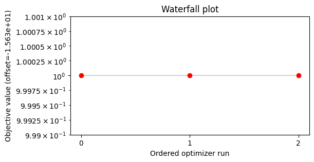
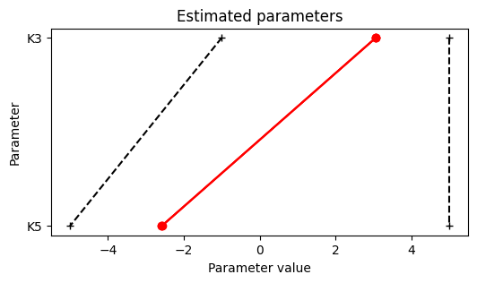
The model optimization has good convergence with a plateu at the optimal point:
[9]:
from pypesto.visualize import parameters, waterfall

waterfall([result], size=(6, 3))
plt.show()
parameters([result], size=(6, 3))
plt.show()
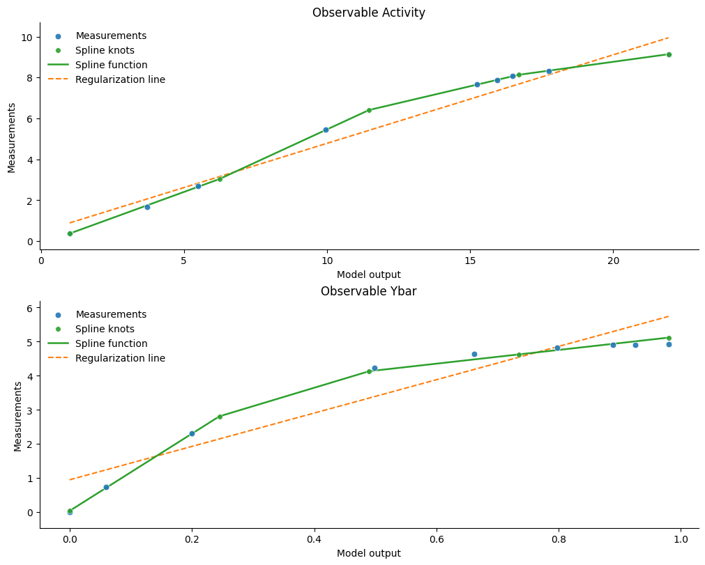
We can visualize the estimated spline observable mapping using the pypesto.visualize.observable_mapping.visualize_estimated_observable_mapping routine. The routine plots all estimated linear or spline observable mappings of relative or semiquantitative observables, respectively.
[10]:
visualize_estimated_observable_mapping(result, problem, figsize=(10, 8))
plt.show()
/home/docs/checkouts/readthedocs.org/user_builds/pypesto/envs/develop/lib/python3.13/site-packages/pypesto/visualize/observable_mapping.py:524: RuntimeWarning: The following problem parameters were not used: {'K2', 'K1'}
  fill_in_parameters(
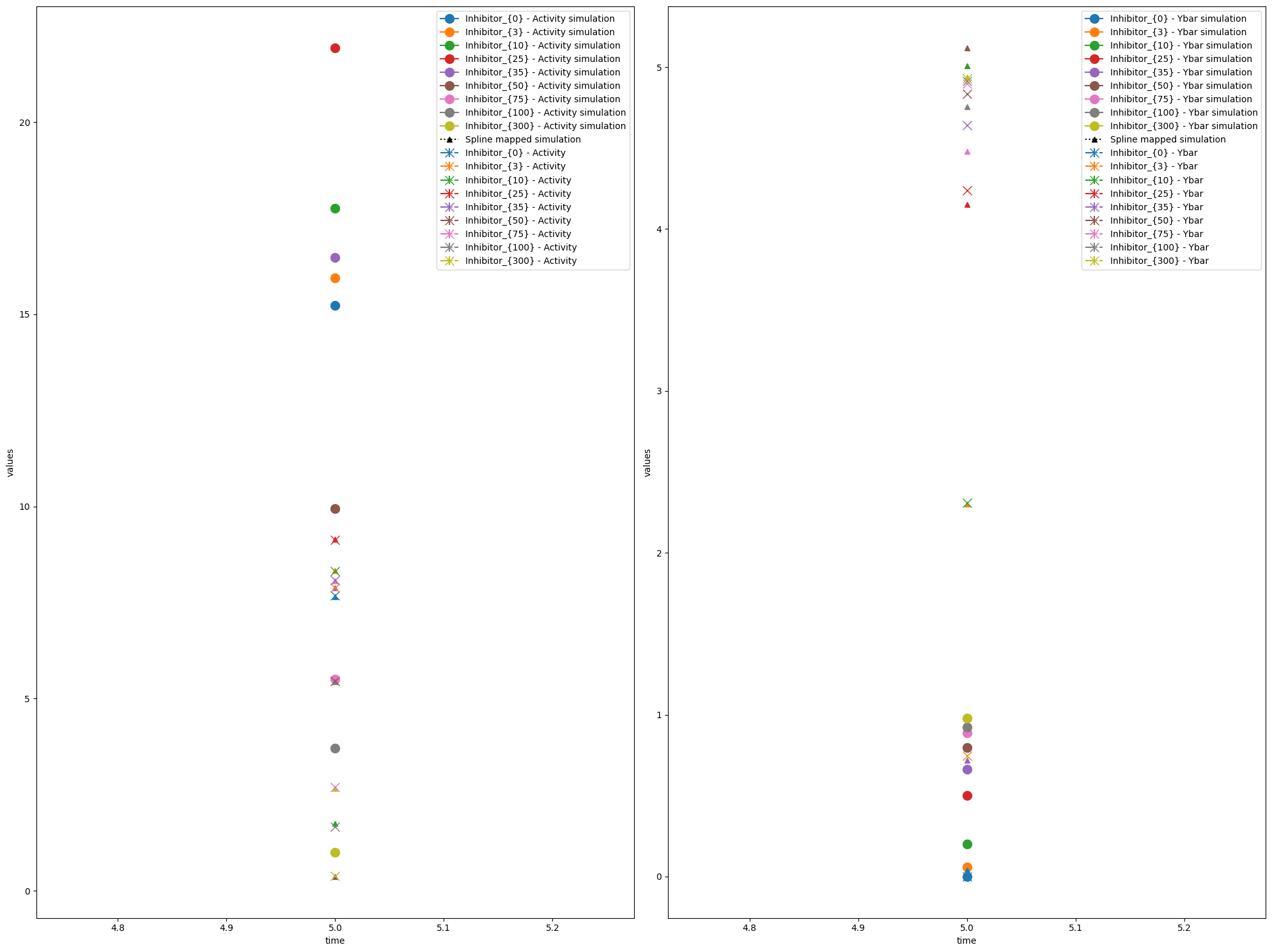
We can also plot the model fit (observable trajectories) with the spline-mapped simulations included using visualize_optimized_model_fit.
[11]:
visualize_optimized_model_fit(
    petab_problem,
    result,
    problem,
)
plt.show()
/home/docs/checkouts/readthedocs.org/user_builds/pypesto/envs/develop/lib/python3.13/site-packages/pypesto/visualize/observable_mapping.py:823: RuntimeWarning: The following problem parameters were not used: {'K2', 'K1'}
  fill_in_parameters(
Caution when using minimal difference
To illustrate that minimal difference sometimes has a negative effect we will apply it to a very simple synthetic “model” – simulation of the exponential function:
[12]:
timepoints = np.linspace(0, 10, 11)
function = np.exp

simulation = timepoints
sigma = np.full(len(timepoints), 1)

# Create synthetic data as the exponential function of timepoints
data = function(timepoints)

spline_ratio = 1 / 2
n_spline_pars = int(np.ceil(spline_ratio * len(timepoints)))


par_type = "spline"
mask = [np.full(len(simulation), True)]

inner_parameters = [
    SplineInnerParameter(
        inner_parameter_id=f"{par_type}_{1}_{par_index + 1}",
        inner_parameter_type=InnerParameterType.SPLINE,
        scale=LIN,
        lb=-np.inf,
        ub=np.inf,
        ixs=mask,
        index=par_index + 1,
        group=1,
        observable_id="observable_1",
    )
    for par_index in range(n_spline_pars)
]

inner_problem = SemiquantProblem(
    xs=inner_parameters, data=[data], edatas=None, spline_ratio=spline_ratio
)

options = {
    "minimal_diff_on": {
        "min_diff_factor": 1 / 2,
    },
    "minimal_diff_off": {
        "min_diff_factor": 0.0,
    },
}
inner_solvers = {}
results = {}

for minimal_diff, option in options.items():
    inner_solvers[minimal_diff] = SemiquantInnerSolver(
        options=option,
    )
    print(f"Using {minimal_diff} options: {option}")

    # Solve the inner problem to obtain the optimal spline
    results[minimal_diff] = inner_solvers[minimal_diff].solve(
        problem=inner_problem,
        sim=[simulation],
        amici_sigma=[sigma],
    )

    plot_splines_from_inner_result(
        inner_problem,
        inner_solvers[minimal_diff],
        results[minimal_diff],
        sim=[simulation],
    )
    plt.show()
Using minimal_diff_on options: {'min_diff_factor': 0.5}
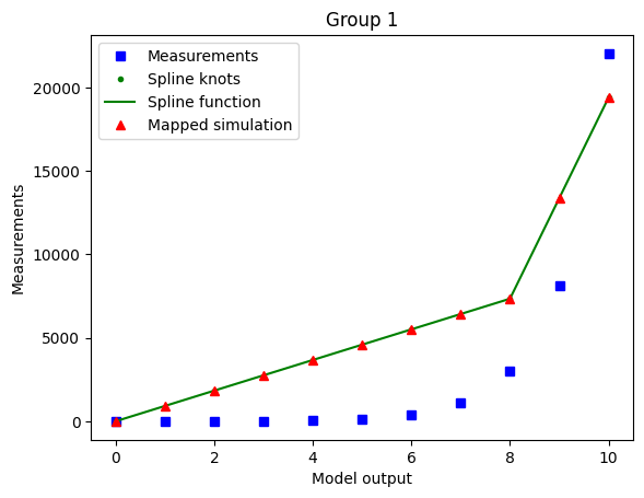
Using minimal_diff_off options: {'min_diff_factor': 0.0}
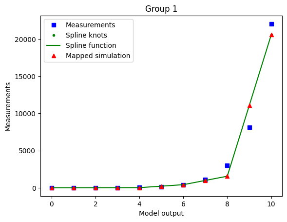
The optimized spline for the case with enabled minimal difference is performing much worse even if we use a non-extreme min_diff_factor value. This is due to the relative flatness of the data with respect to the true model output.
The minimal difference is determined as
so for nonlinear-monotone functions which are relatively flat on some intervals, it is best to keep the minimal difference disabled.
As the true output (e.g. observable simulation of the model with true parameters) is mostly a-priori not known, it’s hard to know whether the minimal difference is going to have a bad or good effect on the optimization. So a good heuristic is to run for different values of min_diff_factor and compare results.