Parameter estimation using censored data
This Notebook explains the use of censored data for parameter estimation of ODE models. An example model is provided in pypesto/doc/example/example_censored. The implementation supports all three censoring types of measurements:
Left censored: a datapoint is below a certain known value.
Right censored: a datapoint is above a certain known value.
Interval censored: a datapoint is on an interval between two known values.
In all three cases, the exact numerical value of the datapoint is unknown. For the integration of censored measurements, we employ the optimal scaling approach. In this approach, each datapoint is represented by a variable surrogate datapoint which is constrained to be in its respective category. Categories can be thought of as intervals with specific bounds.
For censored data, the category bounds are already known from the censoring value:
for left censored data the category bounds are (0, censoring value),
for right censored data the category bounds are (censoring value, infinity),
for interval censored data the category bounds are given by the interval bounds.
This makes the identification of surrogate data extremely simple, as it can be directly (analytically) calculated.
Details on the optimal scaling approach can be found in Shepard, 1962 (https://doi.org/10.1007/BF02289621). Details on the application of the gradient-based optimal scaling approach to mechanistic modeling with ordinal data can be found in Schmiester et al. 2020 (https://doi.org/10.1007/s00285-020-01522-w) and Schmiester et al. 2021 (https://doi.org/10.1093/bioinformatics/btab512).
Import model from the petab_problem
[1]:
import matplotlib.pyplot as plt
import numpy as np
import petab

import pypesto
import pypesto.logging
import pypesto.optimize as optimize
from pypesto.petab import PetabImporter
from pypesto.visualize import plot_categories_from_pypesto_result
To use censored data for parameter estimation, in pyPESTO we use the optimal scaling approach. Since the optimal scaling approach is implemented in the hierarchical manner, it requires us to specify hierarchical=True when importing the petab_problem:
[2]:
petab_folder = './example_censored/'
yaml_file = 'example_censored.yaml'

petab_problem = petab.Problem.from_yaml(petab_folder + yaml_file)

importer = PetabImporter(petab_problem, hierarchical=True)
The petab_problem has to be specified in the usual PEtab formulation. The censored measurements have to be specified in the measurement.tsv file by adding the censoring type in the measurementType column, where a censoring type can be:
left-censored,right-censored,or
interval-censored.
If the censoring type is not specified, the measurement will be considered as quantitative. Then, the censoring bound has to be specified in the censoringBounds column. For interval censored measurements the bounds should be separated with a semicolon:
[3]:
from pandas import option_context

with option_context('display.max_colwidth', 400):
    display(petab_problem.measurement_df)
| observableId | preequilibrationConditionId | simulationConditionId | measurement | time | observableParameters | noiseParameters | observableTransformation | noiseDistribution | measurementType | censoringBounds | |
|---|---|---|---|---|---|---|---|---|---|---|---|
| 0 | Activity | NaN | Inhibitor_0 | 0.000000 | 5 | NaN | 1 | lin | normal | interval-censored | 10.0;16.0 |
| 1 | Activity | NaN | Inhibitor_3 | 0.000000 | 5 | NaN | 1 | lin | normal | interval-censored | 10.0;16.0 |
| 2 | Activity | NaN | Inhibitor_10 | 17.892654 | 5 | NaN | 1 | lin | normal | NaN | NaN |
| 3 | Activity | NaN | Inhibitor_25 | 0.000000 | 5 | NaN | 1 | lin | normal | right-censored | 20.0 |
| 4 | Activity | NaN | Inhibitor_35 | 16.812104 | 5 | NaN | 1 | lin | normal | NaN | NaN |
| 5 | Activity | NaN | Inhibitor_50 | 9.173129 | 5 | NaN | 1 | lin | normal | NaN | NaN |
| 6 | Activity | NaN | Inhibitor_75 | 4.150928 | 5 | NaN | 1 | lin | normal | NaN | NaN |
| 7 | Activity | NaN | Inhibitor_100 | 0.000000 | 5 | NaN | 1 | lin | normal | left-censored | 3.0 |
| 8 | Activity | NaN | Inhibitor_300 | 0.000000 | 5 | NaN | 1 | lin | normal | left-censored | 3.0 |
| 9 | Ybar | NaN | Inhibitor_0 | 0.000000 | 5 | NaN | 1 | lin | normal | NaN | NaN |
| 10 | Ybar | NaN | Inhibitor_3 | 0.059999 | 5 | NaN | 1 | lin | normal | NaN | NaN |
| 11 | Ybar | NaN | Inhibitor_10 | 0.199994 | 5 | NaN | 1 | lin | normal | NaN | NaN |
| 12 | Ybar | NaN | Inhibitor_25 | 0.499043 | 5 | NaN | 1 | lin | normal | NaN | NaN |
| 13 | Ybar | NaN | Inhibitor_35 | 0.659169 | 5 | NaN | 1 | lin | normal | NaN | NaN |
| 14 | Ybar | NaN | Inhibitor_50 | 0.814954 | 5 | NaN | 1 | lin | normal | NaN | NaN |
| 15 | Ybar | NaN | Inhibitor_75 | 0.916383 | 5 | NaN | 1 | lin | normal | NaN | NaN |
| 16 | Ybar | NaN | Inhibitor_100 | 0.948981 | 5 | NaN | 1 | lin | normal | NaN | NaN |
| 17 | Ybar | NaN | Inhibitor_300 | 0.988130 | 5 | NaN | 1 | lin | normal | NaN | NaN |
For censored measurements, the measurement column will be ignored. For the Ybar observable we didn’t specify a measurement type, so those will be used as quantitative.
Note on inclusion of additional data types:
It is possible to include observables with different types of data to the same petab_problem. Refer to the notebooks on using nonlinear-monotone data and ordinal data for details on integration of other data types. Additionally, as shown in this example, if the measurementType column is left empty for all measurements of an observable, the observable will be treated as quantitative.
Construct the objective and pypesto problem
Now when we construct the objective, it will construct all objects of the optimal scaling inner optimization:
OptimalScalingInnerSolverOptimalScalingAmiciCalculatorOptimalScalingProblem
As there are no censored data specific inner options, we will pass none to the constructor.
[4]:
objective = importer.create_objective()
Now let’s construct the pyPESTO problem and optimizer. We’re going to use a gradint-based optimizer for a faster optimization, but gradient-free optimizers can be used in the same way:
[5]:
problem = importer.create_problem(objective)

engine = pypesto.engine.SingleCoreEngine()

optimizer = optimize.ScipyOptimizer(
    method="L-BFGS-B",
    options={"disp": None, "ftol": 2.220446049250313e-09, "gtol": 1e-5},
)
n_starts = 10
np.random.seed(n_starts)
Run optimization using optimal scaling approach
[6]:
np.random.seed(n_starts)

res = optimize.minimize(
    problem, n_starts=n_starts, optimizer=optimizer, engine=engine
)
100%|██████████| 10/10 [00:18<00:00, 1.83s/it]
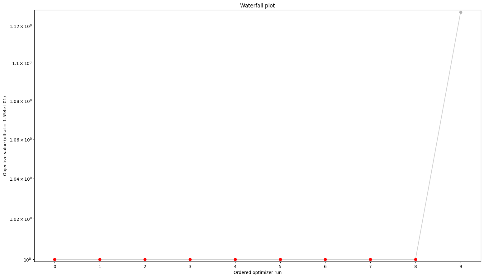
Visualizing the result
[7]:
from pypesto.visualize import waterfall

waterfall(res)
[7]:
<AxesSubplot: title={'center': 'Waterfall plot'}, xlabel='Ordered optimizer run', ylabel='Objective value (offset=-1.554e+01)'>
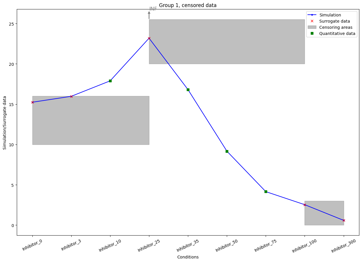
We can plot the censoring categories using the plot_categories_from_pypesto_result plotting function.
[8]:
plot_categories_from_pypesto_result(res, figsize=(15, 10))
plt.show()