Rosenbrock banana
Here, we perform optimization for the Rosenbrock banana function, which does not require an AMICI model. In particular, we try several ways of specifying derivative information.
[1]:
import pypesto
import numpy as np
import scipy as sp
import matplotlib.pyplot as plt
from mpl_toolkits.mplot3d import Axes3D

%matplotlib inline
Define the objective and problem
[2]:
# first type of objective
objective1 = pypesto.Objective(fun=sp.optimize.rosen,
                               grad=sp.optimize.rosen_der,
                               hess=sp.optimize.rosen_hess)

# second type of objective
def rosen2(x):
    return sp.optimize.rosen(x), sp.optimize.rosen_der(x), sp.optimize.rosen_hess(x)
objective2 = pypesto.Objective(fun=rosen2, grad=True, hess=True)

dim_full = 10
lb = -5 * np.ones((dim_full, 1))
ub = 5 * np.ones((dim_full, 1))

problem1 = pypesto.Problem(objective=objective1, lb=lb, ub=ub)
problem2 = pypesto.Problem(objective=objective2, lb=lb, ub=ub)
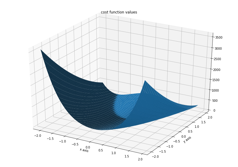
Illustration
[3]:
x = np.arange(-2, 2, 0.1)
y = np.arange(-2, 2, 0.1)
x, y = np.meshgrid(x, y)
z = np.zeros_like(x)
for j in range(0, x.shape[0]):
    for k in range(0, x.shape[1]):
        z[j,k] = objective1([x[j,k], y[j,k]], (0,))
[4]:
fig = plt.figure()
fig.set_size_inches(*(14,10))
ax = plt.axes(projection='3d')
ax.plot_surface(X=x, Y=y, Z=z)
plt.xlabel('x axis')
plt.ylabel('y axis')
ax.set_title('cost function values')
[4]:
Text(0.5, 0.92, 'cost function values')
Run optimization
[5]:
%%time

# create different optimizers
optimizer_bfgs = pypesto.ScipyOptimizer(method='l-bfgs-b')
optimizer_tnc = pypesto.ScipyOptimizer(method='TNC')
optimizer_dogleg = pypesto.ScipyOptimizer(method='dogleg')

# set number of starts
n_starts = 20

# save optimizer trace
history_options = pypesto.HistoryOptions(trace_record=True)

# Run optimizaitons for different optimzers
result1_bfgs = pypesto.minimize(
    problem=problem1, optimizer=optimizer_bfgs,
    n_starts=n_starts, history_options=history_options)
result1_tnc = pypesto.minimize(
    problem=problem1, optimizer=optimizer_tnc,
    n_starts=n_starts, history_options=history_options)
result1_dogleg = pypesto.minimize(
    problem=problem1, optimizer=optimizer_dogleg,
    n_starts=n_starts, history_options=history_options)

# Optimize second type of objective
result2 = pypesto.minimize(problem=problem2, optimizer=optimizer_tnc, n_starts=n_starts)
Function values from history and optimizer do not match: 0.2816653821914888, 0.5320236837009729
Parameters obtained from history and optimizer do not match: [0.98858861 0.98891374 0.98766938 0.98161879 0.9652898  0.93879652
 0.88306125 0.77229682 0.59072196 0.34463656], [0.98496582 0.99181314 0.98908854 0.97887796 0.9637969  0.92698863
 0.85833682 0.7281339  0.5100925  0.23030355]
Function values from history and optimizer do not match: 2.4964418432638706, 3.2754756228142554
Parameters obtained from history and optimizer do not match: [9.82288496e-01 9.66985425e-01 9.38419566e-01 8.78054852e-01
 7.69913490e-01 5.86275734e-01 3.34232174e-01 1.02020372e-01
 1.12463415e-02 8.92327778e-05], [ 9.77936483e-01  9.58866835e-01  9.18622429e-01  8.45125973e-01
  6.98308810e-01  4.68636934e-01  1.81161241e-01  1.56538059e-02
  1.25320748e-02 -3.42245429e-05]
Function values from history and optimizer do not match: 5.2801527327005155, 6.006584566765655
Parameters obtained from history and optimizer do not match: [ 8.97044955e-01  8.02352694e-01  6.38595532e-01  3.92952520e-01
  1.39352250e-01  1.46386081e-02  1.03838418e-02  1.04224904e-02
  9.87858840e-03 -3.10151313e-05], [8.53850657e-01 7.25968721e-01 5.02444501e-01 2.29720701e-01
 2.91937619e-02 1.04279105e-02 1.00588034e-02 9.91318272e-03
 1.01923977e-02 2.48830744e-04]
Function values from history and optimizer do not match: 1.9692004336022721, 2.7115798760594214
Parameters obtained from history and optimizer do not match: [ 0.99019497  0.97774137  0.9561126   0.91685931  0.84524646  0.70666505
  0.49175856  0.23072529  0.03408112 -0.00353803], [ 0.99027014  0.97935022  0.95186067  0.89016816  0.78796339  0.60782056
  0.3439489   0.082957    0.01236261 -0.0090733 ]
Function values from history and optimizer do not match: 8.168889493703478, 8.725825462780923
Parameters obtained from history and optimizer do not match: [-0.94088519  0.89001051  0.79111519  0.61462856  0.36442     0.11619655
  0.01427664  0.01024192  0.00981114  0.0030506 ], [-0.9055118   0.82811563  0.68759974  0.46924951  0.18965995  0.0303
  0.00988695  0.00686135  0.01131552  0.01232474]
Function values from history and optimizer do not match: 5.952343722253962, 6.6703631037412485
Parameters obtained from history and optimizer do not match: [ 8.43835312e-01  7.07958350e-01  4.88024405e-01  2.15876140e-01
  3.61965507e-02  1.06449763e-02  1.02201791e-02  1.01343248e-02
  1.00194415e-02 -4.24013443e-05], [ 7.73014395e-01  5.76458083e-01  3.06751296e-01  7.23116662e-02
  1.11101457e-02  1.04925729e-02  1.02198284e-02  9.31800098e-03
  1.00303338e-02 -3.35414249e-04]
Function values from history and optimizer do not match: 2.9695656384271043, 3.1184191036428834
Parameters obtained from history and optimizer do not match: [9.87034254e-01 9.72306804e-01 9.49987341e-01 8.93423068e-01
 8.17286050e-01 6.40113467e-01 3.50303066e-01 9.21040023e-02
 1.61619582e-02 1.07301208e-05], [0.97539345 0.96038658 0.92103141 0.84071849 0.69173518 0.46411457
 0.22535018 0.02137437 0.0140465  0.00187475]
Function values from history and optimizer do not match: 5.243703633002998, 5.815927741761821
Parameters obtained from history and optimizer do not match: [-0.98596483  0.98274868  0.97442973  0.9514248   0.90830696  0.82066704
  0.6645958   0.42265816  0.16754891  0.00843015], [-9.83776132e-01  9.76891471e-01  9.59822778e-01  9.25805546e-01
  8.61313435e-01  7.38255806e-01  5.36125583e-01  2.68900058e-01
  4.63857306e-02  5.55478747e-04]
Function values from history and optimizer do not match: 5.568452686104578, 6.240940426777619
Parameters obtained from history and optimizer do not match: [-0.98409971  0.97981689  0.96708475  0.93994779  0.882228    0.77067159
  0.58158721  0.3234338   0.08784476  0.00137899], [-9.80621630e-01  9.73220286e-01  9.49144994e-01  8.99631345e-01
  8.13904700e-01  6.72270174e-01  4.38458930e-01  1.59095121e-01
  1.36813582e-02  5.45995408e-04]
Function values from history and optimizer do not match: 0.036324365386529986, 0.09483254249425768
Parameters obtained from history and optimizer do not match: [0.99822004 0.99707243 0.99610909 0.99417929 0.99002028 0.98113164
 0.96153381 0.92444914 0.85179403 0.71878419], [0.99793405 0.9950185  0.99388555 0.99040659 0.98235824 0.966224
 0.93616269 0.87811711 0.77111827 0.58106498]
Function values from history and optimizer do not match: 0.6471617322900747, 1.0298609819176106
Parameters obtained from history and optimizer do not match: [0.99617777 0.9935325  0.98584858 0.97134588 0.94515948 0.88609812
 0.78352677 0.60468994 0.36020607 0.12888943], [0.99486306 0.99041659 0.98198154 0.96653722 0.93323387 0.86752936
 0.75275173 0.55276676 0.2795121  0.04110074]
CPU times: user 4.73 s, sys: 150 ms, total: 4.88 s
Wall time: 4.85 s
Visualize and compare optimization results
[6]:
import pypesto.visualize

# plot separated waterfalls
pypesto.visualize.waterfall(result1_bfgs, size=(15,6))
pypesto.visualize.waterfall(result1_tnc, size=(15,6))
pypesto.visualize.waterfall(result1_dogleg, size=(15,6))
[6]:
<matplotlib.axes._subplots.AxesSubplot at 0x126cfd6a0>
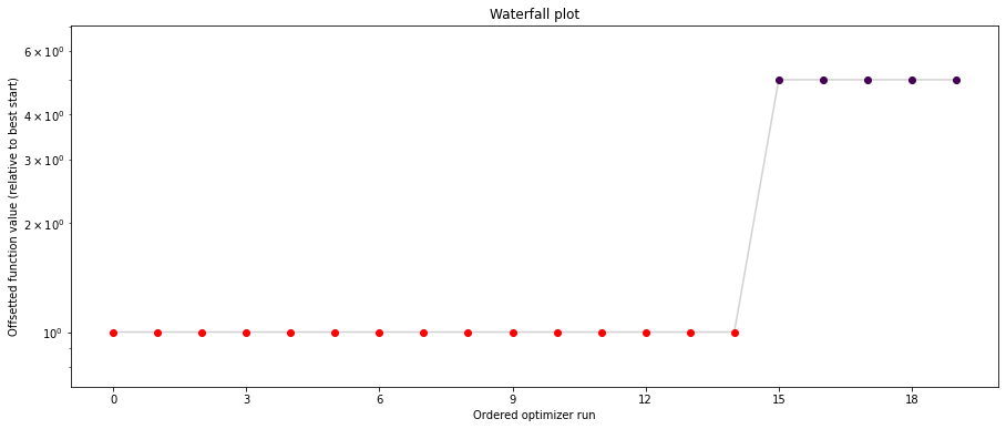
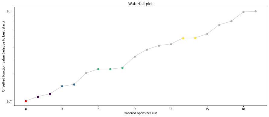
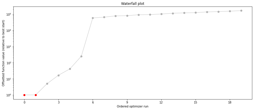
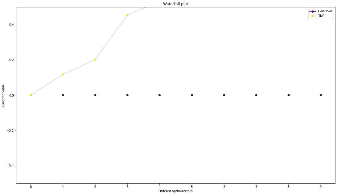
We can now have a closer look, which method perfomred better: Let’s first compare bfgs and TNC, since both methods gave good results. How does the fine convergence look like?
[7]:
# plot one list of waterfalls
pypesto.visualize.waterfall([result1_bfgs, result1_tnc],
                            legends=['L-BFGS-B', 'TNC'],
                            start_indices=10,
                            scale_y='lin')
[7]:
<matplotlib.axes._subplots.AxesSubplot at 0x126ddca00>
[8]:
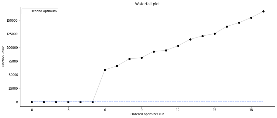
# retrieve second optimum
all_x = result1_bfgs.optimize_result.get_for_key('x')
all_fval = result1_bfgs.optimize_result.get_for_key('fval')
x = all_x[19]
fval = all_fval[19]
print('Second optimum at: ' + str(fval))

# create a reference point from it
ref = {'x': x, 'fval': fval, 'color': [
    0.2, 0.4, 1., 1.], 'legend': 'second optimum'}
ref = pypesto.visualize.create_references(ref)

# new waterfall plot with reference point for second optimum
pypesto.visualize.waterfall(result1_dogleg, size=(15,6),
                            scale_y='lin', y_limits=[-1, 101],
                            reference=ref, colors=[0., 0., 0., 1.])
Second optimum at: 3.986579113118511
[8]:
<matplotlib.axes._subplots.AxesSubplot at 0x1275cbfd0>
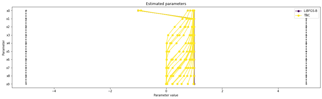
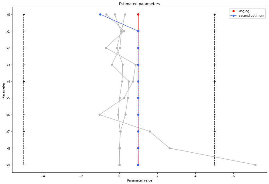
Visualize parameters
There seems to be a second local optimum. We want to see whether it was also found by the dogleg method
[9]:
pypesto.visualize.parameters([result1_bfgs, result1_tnc],
                            legends=['L-BFGS-B', 'TNC'],
                            balance_alpha=False)
pypesto.visualize.parameters(result1_dogleg,
                             legends='dogleg',
                             reference=ref,
                             size=(15,10),
                             start_indices=[0, 1, 2, 3, 4, 5],
                             balance_alpha=False)
[9]:
<matplotlib.axes._subplots.AxesSubplot at 0x1280b3df0>
If the result needs to be examined in more detail, it can easily be exported as a pandas.DataFrame:
[10]:
df = result1_tnc.optimize_result.as_dataframe(
    ['fval', 'n_fval', 'n_grad', 'n_hess', 'n_res', 'n_sres', 'time'])
df.head()
[10]:
| fval | n_fval | n_grad | n_hess | n_res | n_sres | time | |
|---|---|---|---|---|---|---|---|
| 0 | 0.000092 | 101 | 101 | 0 | 0 | 0 | 0.075175 |
| 1 | 0.117351 | 101 | 101 | 0 | 0 | 0 | 0.055569 |
| 2 | 0.201761 | 101 | 101 | 0 | 0 | 0 | 0.089948 |
| 3 | 0.455242 | 101 | 101 | 0 | 0 | 0 | 0.086691 |
| 4 | 0.532024 | 101 | 101 | 0 | 0 | 0 | 0.061193 |
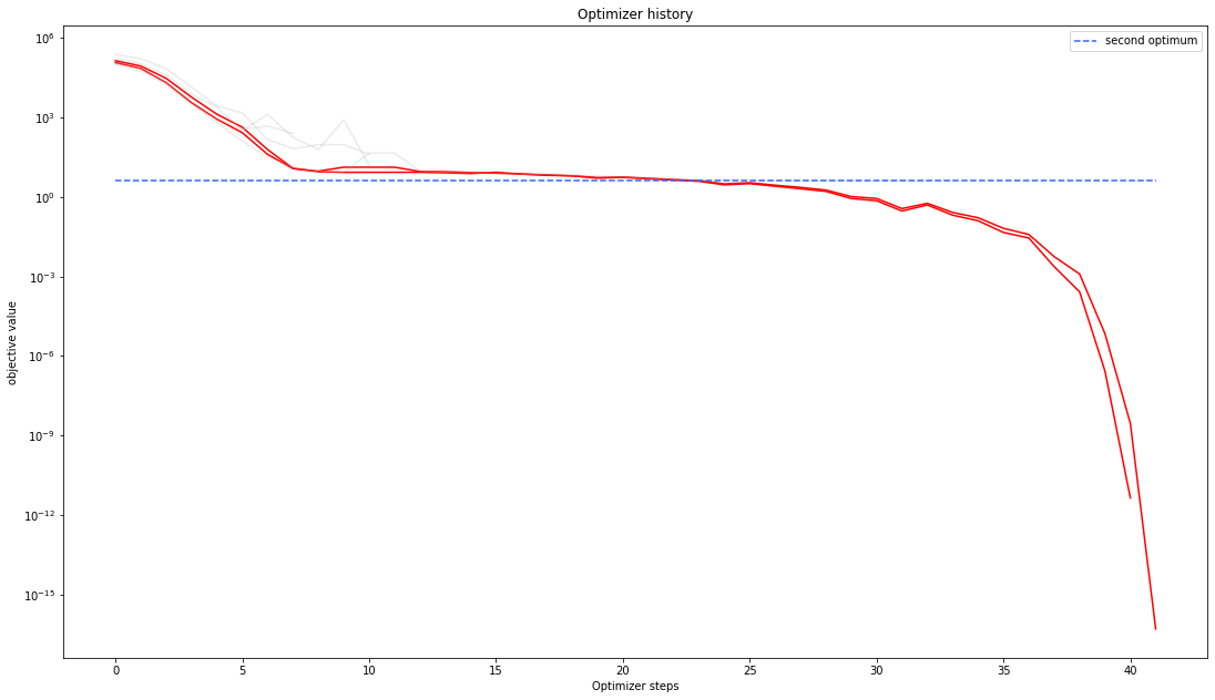
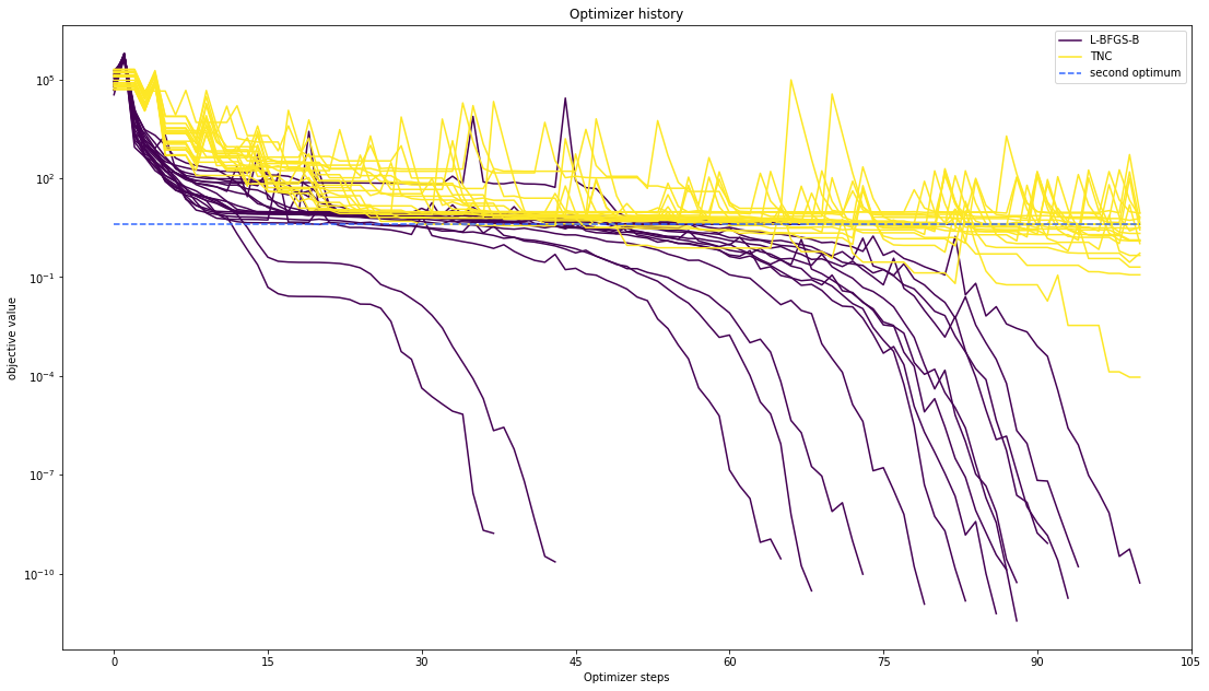
Optimizer history
Let’s compare optimzer progress over time.
[11]:
# plot one list of waterfalls
pypesto.visualize.optimizer_history([result1_bfgs, result1_tnc],
                                    legends=['L-BFGS-B', 'TNC'],
                                    reference=ref)
# plot one list of waterfalls
pypesto.visualize.optimizer_history(result1_dogleg,
                                    reference=ref)
[11]:
<matplotlib.axes._subplots.AxesSubplot at 0x128611c70>

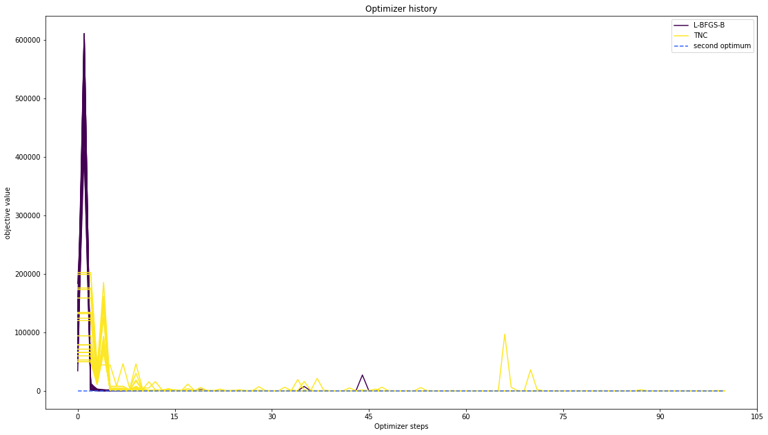
We can also visualize this usign other scalings or offsets…
[12]:
# plot one list of waterfalls
pypesto.visualize.optimizer_history([result1_bfgs, result1_tnc],
                                    legends=['L-BFGS-B', 'TNC'],
                                    reference=ref,
                                    offset_y=0.)

# plot one list of waterfalls
pypesto.visualize.optimizer_history([result1_bfgs, result1_tnc],
                                    legends=['L-BFGS-B', 'TNC'],
                                    reference=ref,
                                    scale_y='lin',
                                    y_limits=[-1., 11.])
[12]:
<matplotlib.axes._subplots.AxesSubplot at 0x129249d90>
Compute profiles
The profiling routine needs a problem, a results object and an optimizer.
Moreover it accepts an index of integer (profile_index), whether or not a profile should be computed.
Finally, an integer (result_index) can be passed, in order to specify the local optimum, from which profiling should be started.
[13]:
%%time

# compute profiles
profile_options = pypesto.ProfileOptions(min_step_size=0.0005,
    delta_ratio_max=0.05,
    default_step_size=0.005,
    ratio_min=0.01)

result1_bfgs = pypesto.parameter_profile(
    problem=problem1,
    result=result1_bfgs,
    optimizer=optimizer_bfgs,
    profile_index=np.array([1, 1, 1, 0, 0, 1, 0, 1, 0, 0, 0]),
    result_index=0,
    profile_options=profile_options)

# compute profiles from second optimum
result1_bfgs = pypesto.parameter_profile(
    problem=problem1,
    result=result1_bfgs,
    optimizer=optimizer_bfgs,
    profile_index=np.array([1, 1, 1, 0, 0, 1, 0, 1, 0, 0, 0]),
    result_index=19,
    profile_options=profile_options)
CPU times: user 2.81 s, sys: 17.2 ms, total: 2.83 s
Wall time: 2.84 s
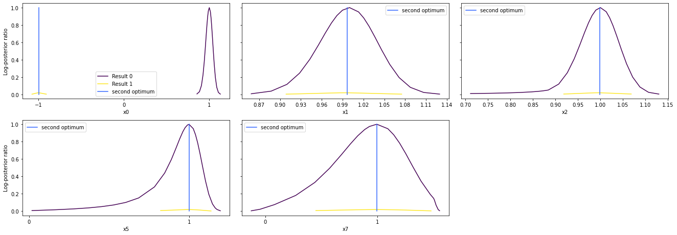
Visualize and analyze results
pypesto offers easy-to-use visualization routines:
[14]:
# specify the parameters, for which profiles should be computed
ax = pypesto.visualize.profiles(result1_bfgs, profile_indices = [0,1,2,5,7],
                           reference=ref, profile_list_ids=[0, 1])
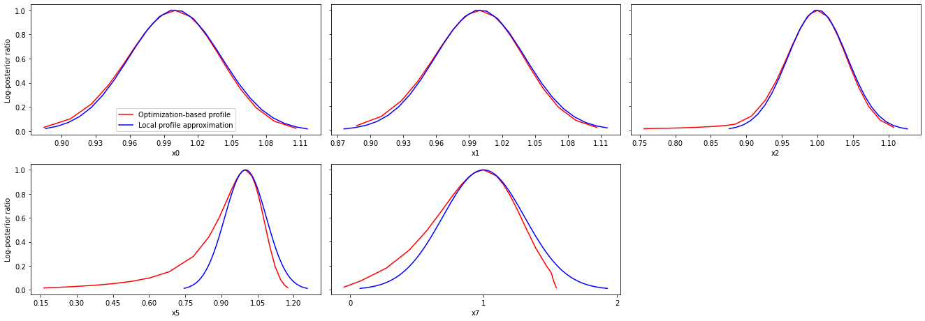
Approximate profiles
When computing the profiles is computationally too demanding, it is possible to employ to at least consider a normal approximation with covariance matrix given by the Hessian or FIM at the optimal parameters.
[15]:
%%time

result1_tnc = pypesto.profile.approximate_parameter_profile(
    problem=problem1,
    result=result1_bfgs,
    profile_index=np.array([1, 1, 1, 0, 0, 1, 0, 1, 0, 0, 0]),
    result_index=0,
    n_steps=1000)
CPU times: user 27.8 ms, sys: 5.92 ms, total: 33.7 ms
Wall time: 20.9 ms
These approximate profiles require at most one additional function evaluation, can however yield substantial approximation errors:
[16]:
axes = pypesto.visualize.profiles(
    result1_bfgs, profile_indices = [0,1,2,5,7], profile_list_ids=[0, 2],
    ratio_min=0.01, colors=[(1,0,0,1), (0,0,1,1)],
    legends=["Optimization-based profile", "Local profile approximation"])
We can also plot approximate confidence intervals based on profiles:
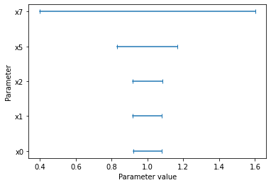
[17]:
pypesto.visualize.profile_cis(result1_bfgs, confidence_level=0.95, profile_list=2)
[17]:
<matplotlib.axes._subplots.AxesSubplot at 0x126ba6a30>