Model import using the Petab format
In this notebook, we illustrate how to use pyPESTO together with PEtab and AMICI. We employ models from the benchmark collection, which we first download:
[1]:
import pypesto
import pypesto.petab
import pypesto.optimize as optimize
import pypesto.visualize as visualize
import amici
import petab

import os
import numpy as np
import matplotlib.pyplot as plt

%matplotlib inline

!git clone --depth 1 https://github.com/Benchmarking-Initiative/Benchmark-Models-PEtab.git tmp/benchmark-models || (cd tmp/benchmark-models && git pull)

folder_base = "tmp/benchmark-models/Benchmark-Models/"
fatal: destination path 'tmp/benchmark-models' already exists and is not an empty directory.
Already up to date.
Import
Manage PEtab model
A PEtab problem comprises all the information on the model, the data and the parameters to perform parameter estimation. We import a model as a petab.Problem.
[2]:
# a collection of models that can be simulated

#model_name = "Zheng_PNAS2012"
model_name = "Boehm_JProteomeRes2014"
#model_name = "Fujita_SciSignal2010"
#model_name = "Sneyd_PNAS2002"
#model_name = "Borghans_BiophysChem1997"
#model_name = "Elowitz_Nature2000"
#model_name = "Crauste_CellSystems2017"
#model_name = "Lucarelli_CellSystems2018"
#model_name = "Schwen_PONE2014"
#model_name = "Blasi_CellSystems2016"

# the yaml configuration file links to all needed files
yaml_config = os.path.join(folder_base, model_name, model_name + '.yaml')

# create a petab problem
petab_problem = petab.Problem.from_yaml(yaml_config)
Import model to AMICI
The model must be imported to pyPESTO and AMICI. Therefore, we create a pypesto.PetabImporter from the problem, and create an AMICI model.
[3]:
importer = pypesto.petab.PetabImporter(petab_problem)

model = importer.create_model()

# some model properties
print("Model parameters:", list(model.getParameterIds()), '\n')
print("Model const parameters:", list(model.getFixedParameterIds()), '\n')
print("Model outputs:   ", list(model.getObservableIds()), '\n')
print("Model states:    ", list(model.getStateIds()), '\n')
Using existing amici model in folder /Users/pauljonasjost/Documents/GitHub_Folders/pyPESTO/doc/example/amici_models/Boehm_JProteomeRes2014.
Model parameters: ['Epo_degradation_BaF3', 'k_exp_hetero', 'k_exp_homo', 'k_imp_hetero', 'k_imp_homo', 'k_phos', 'ratio', 'specC17', 'noiseParameter1_pSTAT5A_rel', 'noiseParameter1_pSTAT5B_rel', 'noiseParameter1_rSTAT5A_rel']

Model const parameters: []

Model outputs:    ['pSTAT5A_rel', 'pSTAT5B_rel', 'rSTAT5A_rel']

Model states:     ['STAT5A', 'STAT5B', 'pApB', 'pApA', 'pBpB', 'nucpApA', 'nucpApB', 'nucpBpB']
Create objective function
To perform parameter estimation, we need to define an objective function, which integrates the model, data, and noise model defined in the PEtab problem.
[4]:
import libsbml
converter_config = libsbml.SBMLLocalParameterConverter()\
    .getDefaultProperties()
petab_problem.sbml_document.convert(converter_config)

obj = importer.create_objective()

# for some models, hyperparamters need to be adjusted
#obj.amici_solver.setMaxSteps(10000)
#obj.amici_solver.setRelativeTolerance(1e-7)
#obj.amici_solver.setAbsoluteTolerance(1e-7)
Using existing amici model in folder /Users/pauljonasjost/Documents/GitHub_Folders/pyPESTO/doc/example/amici_models/Boehm_JProteomeRes2014.
We can request variable derivatives via sensi_orders, or function values or residuals as specified via mode. Passing return_dict, we obtain the direct result of the AMICI simulation.
[5]:
ret = obj(petab_problem.x_nominal_scaled, mode='mode_fun', sensi_orders=(0,1), return_dict=True)
print(ret)
{'fval': 138.22199566457704, 'grad': array([ 2.20546436e-02,  5.53227499e-02,  5.78876640e-03,  5.42272184e-03,
       -4.51595808e-05,  7.91009669e-03,  0.00000000e+00,  1.07876837e-02,
        2.40388572e-02,  1.91925085e-02,  0.00000000e+00]), 'rdatas': [<amici.numpy.ReturnDataView object at 0x7fdb9a293c40>]}
The problem defined in PEtab also defines the fixing of parameters, and parameter bounds. This information is contained in a pypesto.Problem.
[6]:
problem = importer.create_problem(obj)
In particular, the problem accounts for the fixing of parametes.
[7]:
print(problem.x_fixed_indices, problem.x_free_indices)
[6, 10] [0, 1, 2, 3, 4, 5, 7, 8, 9]
The problem creates a copy of he objective function that takes into account the fixed parameters. The objective function is able to calculate function values and derivatives. A finite difference check whether the computed gradient is accurate:
[8]:
objective = problem.objective
ret = objective(petab_problem.x_nominal_free_scaled, sensi_orders=(0,1))
print(ret)
(138.22199566457704, array([ 2.20546436e-02,  5.53227499e-02,  5.78876640e-03,  5.42272184e-03,
       -4.51595808e-05,  7.91009669e-03,  1.07876837e-02,  2.40388572e-02,
        1.91925085e-02]))
[9]:
eps = 1e-4

def fd(x):
    grad = np.zeros_like(x)
    j = 0
    for i, xi in enumerate(x):
        mask = np.zeros_like(x)
        mask[i] += eps
        valinc, _ = objective(x+mask, sensi_orders=(0,1))
        valdec, _ = objective(x-mask, sensi_orders=(0,1))
        grad[j] = (valinc - valdec) / (2*eps)
        j += 1
    return grad

fdval = fd(petab_problem.x_nominal_free_scaled)
print("fd: ", fdval)
print("l2 difference: ", np.linalg.norm(ret[1] - fdval))
fd:  [ 0.02993985  0.05897443 -0.00149735 -0.00281785 -0.00925273  0.01197046
  0.01078638  0.02403756  0.01919121]
l2 difference:  0.017256061672716528
In short
All of the previous steps can be shortened by directly creating an importer object and then a problem:
[10]:
importer = pypesto.petab.PetabImporter.from_yaml(yaml_config)
problem = importer.create_problem()
Using existing amici model in folder /Users/pauljonasjost/Documents/GitHub_Folders/pyPESTO/doc/example/amici_models/Boehm_JProteomeRes2014.
Run optimization
Given the problem, we can perform optimization. We can specify an optimizer to use, and a parallelization engine to speed things up.
[11]:
optimizer = optimize.ScipyOptimizer()

# engine = pypesto.engine.SingleCoreEngine()
engine = pypesto.engine.MultiProcessEngine()

# do the optimization
result = optimize.minimize(problem=problem, optimizer=optimizer,
                           n_starts=10, engine=engine)
Engine set up to use up to 8 processes in total. The number was automatically determined and might not be appropriate on some systems.
Performing parallel task execution on 8 processes.
100%|██████████| 10/10 [00:00<00:00, 131.88it/s]
Using existing amici model in folder /Users/pauljonasjost/Documents/GitHub_Folders/pyPESTO/doc/example/amici_models/Boehm_JProteomeRes2014.
Using existing amici model in folder /Users/pauljonasjost/Documents/GitHub_Folders/pyPESTO/doc/example/amici_models/Boehm_JProteomeRes2014.
Using existing amici model in folder /Users/pauljonasjost/Documents/GitHub_Folders/pyPESTO/doc/example/amici_models/Boehm_JProteomeRes2014.
Using existing amici model in folder /Users/pauljonasjost/Documents/GitHub_Folders/pyPESTO/doc/example/amici_models/Boehm_JProteomeRes2014.
Using existing amici model in folder /Users/pauljonasjost/Documents/GitHub_Folders/pyPESTO/doc/example/amici_models/Boehm_JProteomeRes2014.
Executing task 2.
Using existing amici model in folder /Users/pauljonasjost/Documents/GitHub_Folders/pyPESTO/doc/example/amici_models/Boehm_JProteomeRes2014.
Using existing amici model in folder /Users/pauljonasjost/Documents/GitHub_Folders/pyPESTO/doc/example/amici_models/Boehm_JProteomeRes2014.
Using existing amici model in folder /Users/pauljonasjost/Documents/GitHub_Folders/pyPESTO/doc/example/amici_models/Boehm_JProteomeRes2014.
Executing task 1.
Executing task 0.
Executing task 3.
Executing task 4.
Executing task 6.
Executing task 5.
Executing task 7.
Final fval=249.7460, time=0.3161s, n_fval=20.
Using existing amici model in folder /Users/pauljonasjost/Documents/GitHub_Folders/pyPESTO/doc/example/amici_models/Boehm_JProteomeRes2014.
Final fval=249.7460, time=0.3418s, n_fval=17.
Using existing amici model in folder /Users/pauljonasjost/Documents/GitHub_Folders/pyPESTO/doc/example/amici_models/Boehm_JProteomeRes2014.
Executing task 8.
Executing task 9.
Final fval=249.7460, time=0.6842s, n_fval=39.
[Warning] AMICI:CVODES:CVode:ERR_FAILURE: AMICI ERROR: in module CVODES in function CVode : At t = 116.84 and h = 1.9371e-05, the error test failed repeatedly or with |h| = hmin.
[Warning] AMICI:simulation: AMICI forward simulation failed at t = 116.839896:
AMICI failed to integrate the forward problem

Final fval=159.0527, time=1.7929s, n_fval=102.
[Warning] AMICI:CVODES:CVode:ERR_FAILURE: AMICI ERROR: in module CVODES in function CVode : At t = 89.1085 and h = 1.38467e-05, the error test failed repeatedly or with |h| = hmin.
[Warning] AMICI:simulation: AMICI forward simulation failed at t = 89.108509:
AMICI failed to integrate the forward problem

Final fval=147.5440, time=2.7005s, n_fval=167.
Final fval=156.3410, time=2.5897s, n_fval=136.
Final fval=154.7306, time=2.6399s, n_fval=104.
[Warning] AMICI:CVODES:CVode:ERR_FAILURE: AMICI ERROR: in module CVODES in function CVode : At t = 168.714 and h = 4.02611e-05, the error test failed repeatedly or with |h| = hmin.
[Warning] AMICI:simulation: AMICI forward simulation failed at t = 168.714402:
AMICI failed to integrate the forward problem

Final fval=149.5878, time=3.3350s, n_fval=171.
Final fval=149.5882, time=3.8314s, n_fval=172.
Parameters obtained from history and optimizer do not match: [-1.56379081 -3.2217545   5.          5.         -1.89883736  4.35504207
  0.9094744   0.80931241  1.07766644], [-1.56378624 -3.22180774  5.          5.         -1.89885149  4.355015
  0.9094958   0.80930196  1.07768133]
Final fval=171.1341, time=4.0903s, n_fval=187.
Visualize
The results are contained in a pypesto.Result object. It contains e.g. the optimal function values.
[12]:
result.optimize_result.get_for_key('fval')
[12]:
[147.5440308019394,
 149.5878368928219,
 149.58822002126522,
 154.7306294235784,
 156.3410332994205,
 159.05273185070513,
 171.1340766484108,
 249.74597383547857,
 249.7459974423845,
 249.74599767995497]
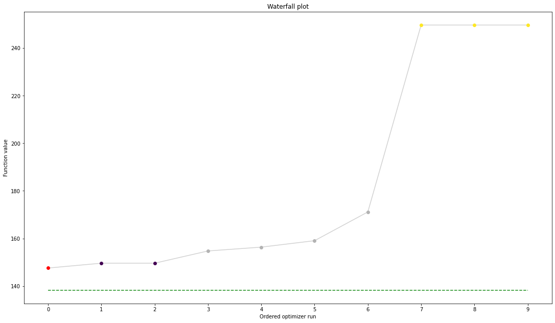
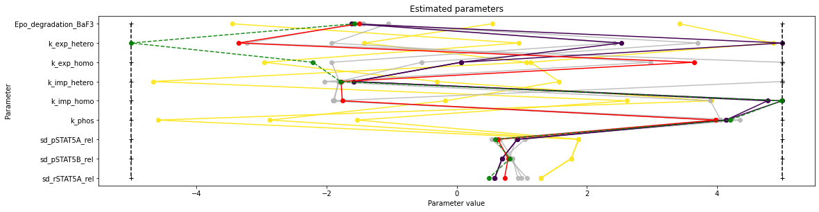
We can use the standard pyPESTO plotting routines to visualize and analyze the results.
[13]:
ref = visualize.create_references(
    x=petab_problem.x_nominal_scaled, fval=obj(petab_problem.x_nominal_scaled))

visualize.waterfall(result, reference=ref, scale_y='lin')
visualize.parameters(result, reference=ref)
[13]:
<AxesSubplot:title={'center':'Estimated parameters'}, xlabel='Parameter value', ylabel='Parameter'>
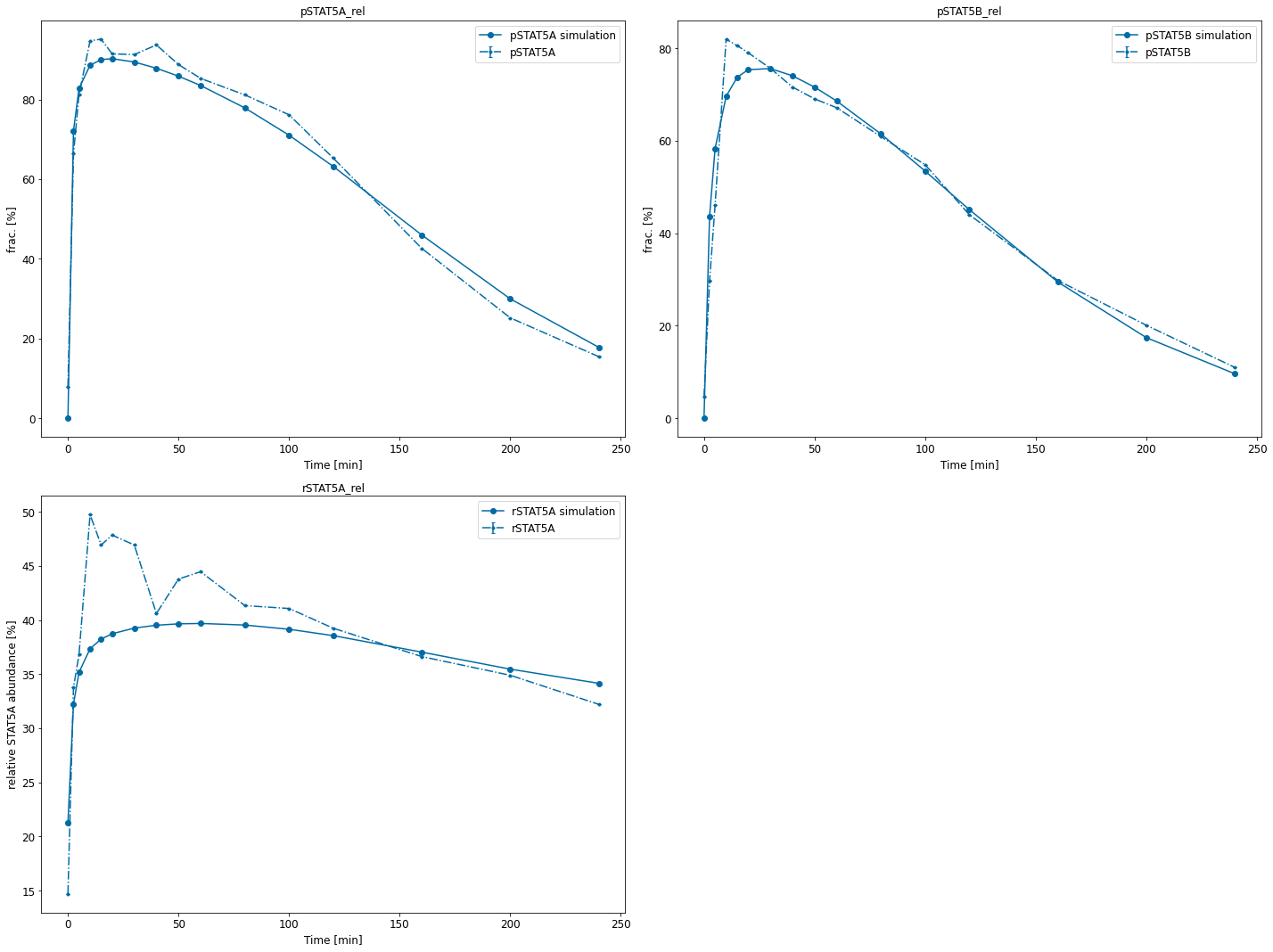
We can also conveniently visualize the model fit. This plots the petab visualization using optimized parameters.
[14]:
# we need to explicitely import the method
from pypesto.visualize.model_fit import visualize_optimized_model_fit
visualize_optimized_model_fit(petab_problem=petab_problem,
                              result=result)
[14]:
{'plot1': <AxesSubplot:title={'center':'pSTAT5A_rel'}, xlabel='Time [min]', ylabel='frac. [%]'>,
 'plot2': <AxesSubplot:title={'center':'pSTAT5B_rel'}, xlabel='Time [min]', ylabel='frac. [%]'>,
 'plot3': <AxesSubplot:title={'center':'rSTAT5A_rel'}, xlabel='Time [min]', ylabel='relative STAT5A abundance [%]'>}