Storage¶

This notebook illustrates how simulations and results can be saved to file.

[1]:

import pypesto
import pypesto.optimize as optimize
import pypesto.visualize as visualize
from pypesto.store import (save_to_hdf5, read_from_hdf5)

import numpy as np
import scipy as sp
import matplotlib.pyplot as plt
import tempfile

%matplotlib inline

Define the objective and problem¶

[2]:

objective = pypesto.Objective(fun=sp.optimize.rosen,
                              grad=sp.optimize.rosen_der,
                              hess=sp.optimize.rosen_hess)

dim_full = 10
lb = -3 * np.ones((dim_full, 1))
ub = 3 * np.ones((dim_full, 1))

problem = pypesto.Problem(objective=objective, lb=lb, ub=ub)

# create optimizers
optimizer = optimize.ScipyOptimizer(method='l-bfgs-b')

# set number of starts
n_starts = 20

Objective function traces¶

During optimization, it is possible to regularly write the objective function trace to file. This is useful e.g. when runs fail, or for various diagnostics. Currently, pyPESTO can save histories to 3 backends: in-memory, as CSV files, or to HDF5 files.

Memory History¶

To record the history in-memory, just set trace_record=True in the pypesto.HistoryOptions. Then, the optimization result contains those histories:

[3]:

# record the history
history_options = pypesto.HistoryOptions(trace_record=True)

# Run optimizaitons
result = optimize.minimize(
    problem=problem, optimizer=optimizer,
    n_starts=n_starts, history_options=history_options)

  0%|          | 0/20 [00:00<?, ?it/s]Executing task 0.
Final fval=0.0000, time=0.0218s, n_fval=94.
Executing task 1.
Final fval=0.0000, time=0.0142s, n_fval=61.
Executing task 2.
Final fval=0.0000, time=0.0191s, n_fval=72.
Executing task 3.
Final fval=0.0000, time=0.0185s, n_fval=76.
Executing task 4.
Final fval=0.0000, time=0.0227s, n_fval=81.
 25%|██▌       | 5/20 [00:00<00:00, 48.89it/s]Executing task 5.
Final fval=0.0000, time=0.0258s, n_fval=83.
Executing task 6.
Final fval=0.0000, time=0.0270s, n_fval=90.
Executing task 7.
Final fval=3.9866, time=0.0278s, n_fval=77.
Executing task 8.
Final fval=0.0000, time=0.0308s, n_fval=98.
Executing task 9.
Final fval=0.0000, time=0.0256s, n_fval=96.
 50%|█████     | 10/20 [00:00<00:00, 39.43it/s]Executing task 10.
Final fval=0.0000, time=0.0224s, n_fval=68.
Executing task 11.
Final fval=0.0000, time=0.0172s, n_fval=64.
Executing task 12.
Final fval=0.0000, time=0.0220s, n_fval=79.
Executing task 13.
Final fval=0.0000, time=0.0277s, n_fval=92.
Executing task 14.
Final fval=0.0000, time=0.0198s, n_fval=70.
 75%|███████▌  | 15/20 [00:00<00:00, 41.09it/s]Executing task 15.
Final fval=0.0000, time=0.0253s, n_fval=81.
Executing task 16.
Final fval=3.9866, time=0.0226s, n_fval=61.
Executing task 17.
Final fval=3.9866, time=0.0307s, n_fval=74.
Executing task 18.
Final fval=3.9866, time=0.0236s, n_fval=71.
Executing task 19.
Final fval=0.0000, time=0.0175s, n_fval=74.
100%|██████████| 20/20 [00:00<00:00, 40.68it/s]

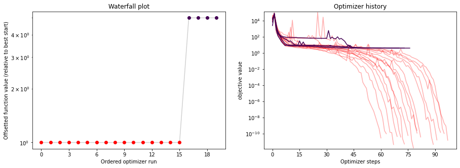
Now, in addition to queries on the result, we can also access the

[4]:

print("History type: ", type(result.optimize_result.list[0].history))
# print("Function value trace of best run: ", result.optimize_result.list[0].history.get_fval_trace())

fig, ax = plt.subplots(1, 2)
visualize.waterfall(result, ax=ax[0])
visualize.optimizer_history(result, ax=ax[1])
fig.set_size_inches((15, 5))

History type:  <class 'pypesto.objective.history.MemoryHistory'>

CSV History¶

The in-memory storage is however not stored anywhere. To do that, it is possible to store either to CSV or HDF5. This is specified via the storage_file option. If it ends in .csv, a pypesto.objective.history.CsvHistory will be employed; if it ends in .hdf5 a pypesto.objective.history.Hdf5History. Occurrences of the substring {id} in the filename are replaced by the multistart id, allowing to maintain a separate file per run (this is necessary for CSV as otherwise runs are overwritten).

[5]:

# record the history and store to CSV
history_options = pypesto.HistoryOptions(trace_record=True, storage_file='history_{id}.csv')

# Run optimizaitons
result = optimize.minimize(
    problem=problem, optimizer=optimizer,
    n_starts=n_starts, history_options=history_options)

  0%|          | 0/20 [00:00<?, ?it/s]Executing task 0.
Final fval=0.0000, time=1.3848s, n_fval=87.
  5%|▌         | 1/20 [00:01<00:26,  1.39s/it]Executing task 1.
Final fval=0.0000, time=1.0376s, n_fval=66.
 10%|█         | 2/20 [00:02<00:21,  1.18s/it]Executing task 2.
Final fval=0.0000, time=1.3995s, n_fval=87.
 15%|█▌        | 3/20 [00:03<00:21,  1.28s/it]Executing task 3.
Final fval=0.0000, time=1.3883s, n_fval=87.
 20%|██        | 4/20 [00:05<00:21,  1.33s/it]Executing task 4.
Final fval=0.0000, time=1.1283s, n_fval=74.
 25%|██▌       | 5/20 [00:06<00:18,  1.25s/it]Executing task 5.
Final fval=0.0000, time=1.2335s, n_fval=81.
 30%|███       | 6/20 [00:07<00:17,  1.25s/it]Executing task 6.
Final fval=3.9866, time=1.6121s, n_fval=106.
 35%|███▌      | 7/20 [00:09<00:17,  1.37s/it]Executing task 7.
Final fval=0.0000, time=1.2220s, n_fval=77.
 40%|████      | 8/20 [00:10<00:15,  1.32s/it]Executing task 8.
Final fval=0.0000, time=1.0812s, n_fval=71.
 45%|████▌     | 9/20 [00:11<00:13,  1.25s/it]Executing task 9.
Final fval=0.0000, time=1.5227s, n_fval=78.
 50%|█████     | 10/20 [00:13<00:13,  1.33s/it]Executing task 10.
Final fval=0.0000, time=1.9653s, n_fval=97.
 55%|█████▌    | 11/20 [00:14<00:13,  1.53s/it]Executing task 11.
Final fval=0.0000, time=1.9667s, n_fval=94.
 60%|██████    | 12/20 [00:16<00:13,  1.66s/it]Executing task 12.
Final fval=0.0000, time=1.0537s, n_fval=57.
 65%|██████▌   | 13/20 [00:18<00:10,  1.48s/it]Executing task 13.
Final fval=0.0000, time=1.5494s, n_fval=81.
 70%|███████   | 14/20 [00:19<00:09,  1.50s/it]Executing task 14.
Final fval=0.0000, time=1.8838s, n_fval=94.
 75%|███████▌  | 15/20 [00:21<00:08,  1.62s/it]Executing task 15.
Final fval=0.0000, time=1.8472s, n_fval=84.
 80%|████████  | 16/20 [00:23<00:06,  1.69s/it]Executing task 16.
Final fval=0.0000, time=1.6928s, n_fval=85.
 85%|████████▌ | 17/20 [00:25<00:05,  1.69s/it]Executing task 17.
Final fval=0.0000, time=1.4911s, n_fval=83.
 90%|█████████ | 18/20 [00:26<00:03,  1.63s/it]Executing task 18.
Final fval=0.0000, time=1.3229s, n_fval=74.
 95%|█████████▌| 19/20 [00:27<00:01,  1.54s/it]Executing task 19.
Final fval=0.0000, time=1.5840s, n_fval=79.
100%|██████████| 20/20 [00:29<00:00,  1.47s/it]

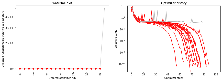
Note that for this simple cost function, saving to CSV takes a considerable amount of time. This overhead decreases for more costly simulators, e.g. using ODE simulations via AMICI.

[6]:

print("History type: ", type(result.optimize_result.list[0].history))
# print("Function value trace of best run: ", result.optimize_result.list[0].history.get_fval_trace())

fig, ax = plt.subplots(1, 2)
visualize.waterfall(result, ax=ax[0])
visualize.optimizer_history(result, ax=ax[1])
fig.set_size_inches((15, 5))

History type:  <class 'pypesto.objective.history.CsvHistory'>

HDF5 History¶

Just as in CSV, writing the history to HDF5 takes a considerable amount of time. If a user specifies a HDF5 output file named my_results.hdf5 and uses a parallelization engine, then: * a folder is created to contain partial results, named my_results/ (the stem of the output filename) * files are created to store the results of each start, named my_results/my_results_{START_INDEX}.hdf5 * a file is created to store the combined result from all starts, named my_results.hdf5. Note that this file depends on the files in the my_results/ directory, so cease to function if my_results/ is deleted.

[7]:

# record the history and store to CSV
history_options = pypesto.HistoryOptions(trace_record=True, storage_file='history.hdf5')

# Run optimizaitons
result = optimize.minimize(
    problem=problem, optimizer=optimizer,
    n_starts=n_starts, history_options=history_options)

  0%|          | 0/20 [00:00<?, ?it/s]Executing task 0.
Final fval=0.0000, time=0.5606s, n_fval=322.
  5%|▌         | 1/20 [00:00<00:10,  1.78it/s]Executing task 1.
Final fval=3.9866, time=0.3860s, n_fval=280.
 10%|█         | 2/20 [00:00<00:08,  2.18it/s]Executing task 2.
Final fval=0.0000, time=0.5257s, n_fval=342.
 15%|█▌        | 3/20 [00:01<00:08,  2.04it/s]Executing task 3.
Final fval=0.0000, time=0.4912s, n_fval=333.
 20%|██        | 4/20 [00:01<00:07,  2.04it/s]Executing task 4.
Final fval=3.9866, time=0.3889s, n_fval=324.
 25%|██▌       | 5/20 [00:02<00:06,  2.20it/s]Executing task 5.
Final fval=0.0000, time=0.4808s, n_fval=345.
 30%|███       | 6/20 [00:02<00:06,  2.15it/s]Executing task 6.
Final fval=0.0000, time=0.4517s, n_fval=322.
 35%|███▌      | 7/20 [00:03<00:05,  2.17it/s]Executing task 7.
Final fval=0.0000, time=0.5006s, n_fval=347.
 40%|████      | 8/20 [00:03<00:05,  2.11it/s]Executing task 8.
Final fval=0.0000, time=0.4723s, n_fval=311.
 45%|████▌     | 9/20 [00:04<00:05,  2.11it/s]Executing task 9.
Final fval=0.0000, time=0.3521s, n_fval=307.
 50%|█████     | 10/20 [00:04<00:04,  2.29it/s]Executing task 10.
Final fval=3.9866, time=0.4401s, n_fval=283.
 55%|█████▌    | 11/20 [00:05<00:03,  2.28it/s]Executing task 11.
Final fval=0.0000, time=0.4453s, n_fval=356.
 60%|██████    | 12/20 [00:05<00:03,  2.27it/s]Executing task 12.
Final fval=0.0000, time=0.3788s, n_fval=335.
 65%|██████▌   | 13/20 [00:05<00:02,  2.37it/s]Executing task 13.
Final fval=0.0000, time=0.4477s, n_fval=334.
 70%|███████   | 14/20 [00:06<00:02,  2.32it/s]Executing task 14.
Final fval=0.0000, time=0.4339s, n_fval=319.
 75%|███████▌  | 15/20 [00:06<00:02,  2.31it/s]Executing task 15.
Final fval=0.0000, time=0.4260s, n_fval=343.
 80%|████████  | 16/20 [00:07<00:01,  2.32it/s]Executing task 16.
Final fval=3.9866, time=0.4394s, n_fval=313.
 85%|████████▌ | 17/20 [00:07<00:01,  2.31it/s]Executing task 17.
Final fval=0.0000, time=0.2605s, n_fval=265.
 90%|█████████ | 18/20 [00:07<00:00,  2.62it/s]Executing task 18.
Final fval=0.0000, time=0.4477s, n_fval=340.
 95%|█████████▌| 19/20 [00:08<00:00,  2.49it/s]Executing task 19.
Final fval=3.9866, time=0.5053s, n_fval=337.
100%|██████████| 20/20 [00:08<00:00,  2.26it/s]

[8]:

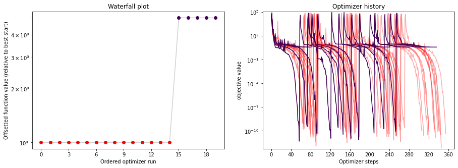
print("History type: ", type(result.optimize_result.list[0].history))
# print("Function value trace of best run: ", result.optimize_result.list[0].history.get_fval_trace())

fig, ax = plt.subplots(1, 2)
visualize.waterfall(result, ax=ax[0])
visualize.optimizer_history(result, ax=ax[1])
fig.set_size_inches((15, 5))

History type:  <class 'pypesto.objective.history.Hdf5History'>

Result storage¶

Result objects can be stored as HDF5 files. When applicable, this is preferable to just pickling results, which is not guaranteed to be reproducible in the future.

[9]:

# Run optimizaitons
result = optimize.minimize(
    problem=problem, optimizer=optimizer,
    n_starts=n_starts)

  0%|          | 0/20 [00:00<?, ?it/s]Executing task 0.
Final fval=3.9866, time=0.0118s, n_fval=48.
Executing task 1.
Final fval=3.9866, time=0.0201s, n_fval=90.
Executing task 2.
Final fval=0.0000, time=0.0210s, n_fval=100.
Executing task 3.
Final fval=0.0000, time=0.0164s, n_fval=73.
Executing task 4.
Final fval=0.0000, time=0.0174s, n_fval=76.
Executing task 5.
Final fval=0.0000, time=0.0155s, n_fval=71.
 30%|███       | 6/20 [00:00<00:00, 55.46it/s]Executing task 6.
Final fval=0.0000, time=0.0190s, n_fval=87.
Executing task 7.
Final fval=0.0000, time=0.0195s, n_fval=88.
Executing task 8.
Final fval=0.0000, time=0.0177s, n_fval=79.
Executing task 9.
Final fval=3.9866, time=0.0179s, n_fval=83.
Executing task 10.
Final fval=0.0000, time=0.0188s, n_fval=86.
Executing task 11.
Final fval=3.9866, time=0.0202s, n_fval=84.
 60%|██████    | 12/20 [00:00<00:00, 52.23it/s]Executing task 12.
Final fval=3.9866, time=0.0188s, n_fval=82.
Executing task 13.
Final fval=0.0000, time=0.0211s, n_fval=91.
Executing task 14.
Final fval=3.9866, time=0.0170s, n_fval=75.
Executing task 15.
Final fval=0.0000, time=0.0124s, n_fval=54.
Executing task 16.
Final fval=0.0000, time=0.0161s, n_fval=70.
Executing task 17.
Final fval=0.0000, time=0.0177s, n_fval=81.
 90%|█████████ | 18/20 [00:00<00:00, 53.48it/s]Executing task 18.
Final fval=0.0000, time=0.0187s, n_fval=82.
Executing task 19.
Final fval=3.9866, time=0.0163s, n_fval=75.
100%|██████████| 20/20 [00:00<00:00, 53.45it/s]

[10]:

result.optimize_result.list[0:2]

[10]:

[{'id': '4',
  'x': array([1.00000001, 1.        , 1.        , 0.99999999, 0.99999999,
         1.00000001, 1.00000001, 1.00000004, 1.00000008, 1.00000014]),
  'fval': 2.6045655152986313e-13,
  'grad': array([ 7.38459033e-06, -4.78320167e-07, -6.50914679e-07, -1.47726642e-06,
         -1.39575141e-05,  9.14793168e-06, -7.58437136e-06,  4.50055738e-07,
          1.01219510e-05, -4.24214104e-06]),
  'hess': None,
  'res': None,
  'sres': None,
  'n_fval': 76,
  'n_grad': 76,
  'n_hess': 0,
  'n_res': 0,
  'n_sres': 0,
  'x0': array([ 0.33383114,  2.09297901, -1.77381628, -1.60663808, -2.85350433,
          0.71050093, -1.190691  ,  0.91974885, -2.34344618,  1.21791823]),
  'fval0': 18119.670540771178,
  'history': <pypesto.objective.history.History at 0x7ffd399536a0>,
  'exitflag': 0,
  'time': 0.017375946044921875,
  'message': 'CONVERGENCE: REL_REDUCTION_OF_F_<=_FACTR*EPSMCH'},
 {'id': '16',
  'x': array([1.        , 1.        , 1.00000001, 1.        , 1.00000001,
         1.00000003, 1.00000007, 1.00000009, 1.00000017, 1.00000039]),
  'fval': 7.312572536347769e-13,
  'grad': array([ 3.34432881e-06, -6.16413761e-06,  1.25983886e-05, -5.34613024e-06,
         -7.50765648e-06,  1.11777438e-06,  1.94167105e-05, -5.91496342e-06,
         -2.50337361e-05,  1.19659990e-05]),
  'hess': None,
  'res': None,
  'sres': None,
  'n_fval': 70,
  'n_grad': 70,
  'n_hess': 0,
  'n_res': 0,
  'n_sres': 0,
  'x0': array([ 2.58291438,  2.48719491,  2.93132676, -0.75290073,  0.34568409,
          0.60255167, -0.68200823, -1.01952663, -2.47953741,  2.14959561]),
  'fval0': 14770.270006296314,
  'history': <pypesto.objective.history.History at 0x7ffd496cea90>,
  'exitflag': 0,
  'time': 0.016092777252197266,
  'message': 'CONVERGENCE: REL_REDUCTION_OF_F_<=_FACTR*EPSMCH'}]

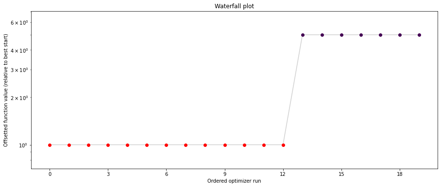
As usual, having obtained our result, we can directly perform some plots:

[11]:

# plot waterfalls
visualize.waterfall(result, size=(15,6))

[11]:

<AxesSubplot:title={'center':'Waterfall plot'}, xlabel='Ordered optimizer run', ylabel='Offsetted function value (relative to best start)'>

Save optimization result as HDF5 file¶

The optimization result can be saved with pypesto.store.write_result(). This will write the problem and the optimization result, and the profiling and sampling results if available, to HDF5. All of them can be disabled with boolean flags (see the documentation)

[12]:

fn = tempfile.mktemp(".hdf5")

# Write result
save_to_hdf5.write_result(result, fn)

Warning: There is no sampling_result, which you tried to save to hdf5.

Read optimization result from HDF5 file¶

When reading in the stored result again, we recover the original optimization result:

[13]:

# Read result and problem
result = read_from_hdf5.read_result(fn)

WARNING: You are loading a problem.
This problem is not to be used without a separately created objective.
WARNING: You are loading a problem.
This problem is not to be used without a separately created objective.
WARNING: You are loading a problem.
This problem is not to be used without a separately created objective.
WARNING: You are loading a problem.
This problem is not to be used without a separately created objective.
Loading the sampling result failed. It is highly likely that no sampling result exists within /var/folders/2f/bnywv1ns2_9g8wtzlf_74yzh0000gn/T/tmpewjf65r6.hdf5.

[14]:

result.optimize_result.list[0:2]

[14]:

[{'id': '4',
  'x': array([1.00000001, 1.        , 1.        , 0.99999999, 0.99999999,
         1.00000001, 1.00000001, 1.00000004, 1.00000008, 1.00000014]),
  'fval': 2.6045655152986313e-13,
  'grad': array([ 7.38459033e-06, -4.78320167e-07, -6.50914679e-07, -1.47726642e-06,
         -1.39575141e-05,  9.14793168e-06, -7.58437136e-06,  4.50055738e-07,
          1.01219510e-05, -4.24214104e-06]),
  'hess': None,
  'res': None,
  'sres': None,
  'n_fval': 76,
  'n_grad': 76,
  'n_hess': 0,
  'n_res': 0,
  'n_sres': 0,
  'x0': array([ 0.33383114,  2.09297901, -1.77381628, -1.60663808, -2.85350433,
          0.71050093, -1.190691  ,  0.91974885, -2.34344618,  1.21791823]),
  'fval0': 18119.670540771178,
  'history': None,
  'exitflag': 0,
  'time': 0.017375946044921875,
  'message': 'CONVERGENCE: REL_REDUCTION_OF_F_<=_FACTR*EPSMCH'},
 {'id': '16',
  'x': array([1.        , 1.        , 1.00000001, 1.        , 1.00000001,
         1.00000003, 1.00000007, 1.00000009, 1.00000017, 1.00000039]),
  'fval': 7.312572536347769e-13,
  'grad': array([ 3.34432881e-06, -6.16413761e-06,  1.25983886e-05, -5.34613024e-06,
         -7.50765648e-06,  1.11777438e-06,  1.94167105e-05, -5.91496342e-06,
         -2.50337361e-05,  1.19659990e-05]),
  'hess': None,
  'res': None,
  'sres': None,
  'n_fval': 70,
  'n_grad': 70,
  'n_hess': 0,
  'n_res': 0,
  'n_sres': 0,
  'x0': array([ 2.58291438,  2.48719491,  2.93132676, -0.75290073,  0.34568409,
          0.60255167, -0.68200823, -1.01952663, -2.47953741,  2.14959561]),
  'fval0': 14770.270006296314,
  'history': None,
  'exitflag': 0,
  'time': 0.016092777252197266,
  'message': 'CONVERGENCE: REL_REDUCTION_OF_F_<=_FACTR*EPSMCH'}]

[15]:

# plot waterfalls
pypesto.visualize.waterfall(result, size=(15,6))

[15]:

<AxesSubplot:title={'center':'Waterfall plot'}, xlabel='Ordered optimizer run', ylabel='Offsetted function value (relative to best start)'>