Conversion reaction
[1]:
import importlib
import os
import sys
import numpy as np
import amici
import amici.plotting
import pypesto
import pypesto.optimize as optimize
import pypesto.visualize as visualize

# sbml file we want to import
sbml_file = 'conversion_reaction/model_conversion_reaction.xml'
# name of the model that will also be the name of the python module
model_name = 'model_conversion_reaction'
# directory to which the generated model code is written
model_output_dir = 'tmp/' + model_name
Compile AMICI model
[2]:
# import sbml model, compile and generate amici module
sbml_importer = amici.SbmlImporter(sbml_file)
sbml_importer.sbml2amici(model_name,
                         model_output_dir,
                         verbose=False)
Load AMICI model
[3]:
# load amici module (the usual starting point later for the analysis)
sys.path.insert(0, os.path.abspath(model_output_dir))
model_module = importlib.import_module(model_name)
model = model_module.getModel()
model.requireSensitivitiesForAllParameters()
model.setTimepoints(np.linspace(0, 10, 11))
model.setParameterScale(amici.ParameterScaling.log10)
model.setParameters([-0.3,-0.7])
solver = model.getSolver()
solver.setSensitivityMethod(amici.SensitivityMethod.forward)
solver.setSensitivityOrder(amici.SensitivityOrder.first)
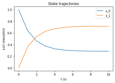
# how to run amici now:
rdata = amici.runAmiciSimulation(model, solver, None)
amici.plotting.plotStateTrajectories(rdata)
edata = amici.ExpData(rdata, 0.2, 0.0)
Optimize
[4]:
# create objective function from amici model
# pesto.AmiciObjective is derived from pesto.Objective,
# the general pesto objective function class
objective = pypesto.AmiciObjective(model, solver, [edata], 1)

# create optimizer object which contains all information for doing the optimization
optimizer = optimize.ScipyOptimizer(method='ls_trf')

# create problem object containing all information on the problem to be solved
problem = pypesto.Problem(objective=objective,
                          lb=[-2,-2], ub=[2,2])

# do the optimization
result = optimize.minimize(problem=problem,
                           optimizer=optimizer,
                           n_starts=10)
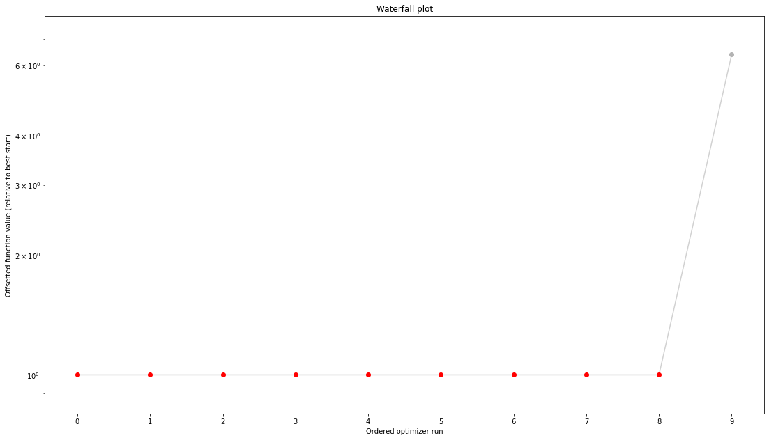
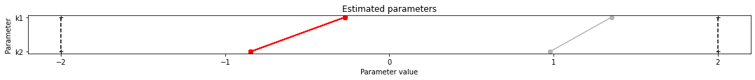
Visualize
[5]:
visualize.waterfall(result)
visualize.parameters(result)
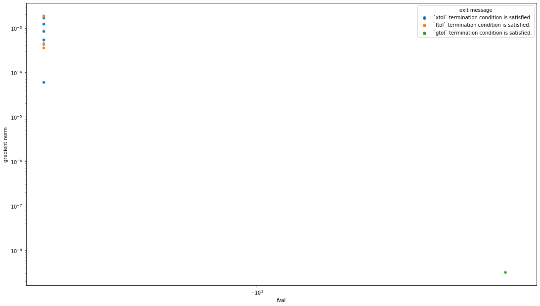
visualize.optimizer_convergence(result)
[5]:
<AxesSubplot:xlabel='fval', ylabel='gradient norm'>
Profiles
[6]:
import pypesto.profile as profile

profile_options = profile.ProfileOptions(min_step_size=0.0005,
    delta_ratio_max=0.05,
    default_step_size=0.005,
    ratio_min=0.01)

result = profile.parameter_profile(
    problem=problem,
    result=result,
    optimizer=optimizer,
    profile_index=np.array([1, 1, 1, 0, 0, 1, 0, 1, 0, 0, 0]),
    result_index=0,
    profile_options=profile_options)
Parameters obtained from history and optimizer do not match: [-0.17103023], [-0.17102486]
Parameters obtained from history and optimizer do not match: [-0.92272262], [-0.92270649]
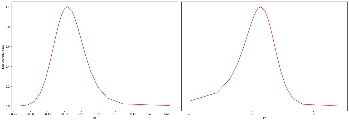
[7]:
# specify the parameters, for which profiles should be computed
ax = visualize.profiles(result)
Sampling
[8]:
import pypesto.sample as sample

sampler = sample.AdaptiveParallelTemperingSampler(
    internal_sampler=sample.AdaptiveMetropolisSampler(),
    n_chains=3)

result = sample.sample(problem, n_samples=10000, sampler=sampler, result=result)
100%|██████████| 10000/10000 [00:33<00:00, 295.74it/s]
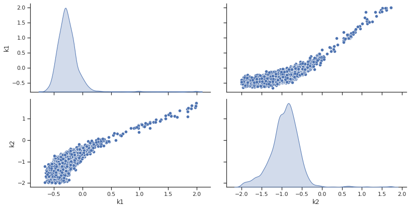
[9]:
ax = visualize.sampling_scatter(result, size=[13,6])
Burn in index not found in the results, the full chain will be shown.
You may want to use, e.g., 'pypesto.sample.geweke_test'.
Predict
[10]:
# Let's create a function, which predicts the ratio of x_1 and x_0
import pypesto.predict as predict

def ratio_function(amici_output_list):
    # This (optional) function post-processes the results from AMICI and must accept one input:
    # a list of dicts, with the fields t, x, y[, sx, sy - if sensi_orders includes 1]
    # We need to specify the simulation condition: here, we only have one, i.e., it's [0]
    x = amici_output_list[0]['x']
    ratio = x[:,1] / x[:,0]
    # we need to output also at least one simulation condition
    return [ratio]

# create pypesto prediction function
predictor = predict.AmiciPredictor(objective, post_processor=ratio_function, output_ids=['ratio'])

# run prediction
prediction = predictor(x=model.getUnscaledParameters())
[11]:
dict(prediction)
[11]:
{'conditions': [{'timepoints': array([ 0.,  1.,  2.,  3.,  4.,  5.,  6.,  7.,  8.,  9., 10.]),
   'output_ids': ['ratio'],
   'x_names': ['k1', 'k2'],
   'output': array([0.        , 1.95196396, 2.00246152, 2.00290412, 2.00290796,
          2.00290801, 2.00290801, 2.00290799, 2.002908  , 2.00290801,
          2.002908  ]),
   'output_sensi': None}],
 'condition_ids': ['condition_0'],
 'comment': None,
 'parameter_ids': ['k1', 'k2']}
Analyze parameter ensembles
[12]:
# We want to use the sample result to create a prediction
from pypesto.ensemble import ensemble

# first collect some vectors from the sampling result
vectors = result.sample_result.trace_x[0, ::20, :]

# create the collection
my_ensemble = ensemble.Ensemble(vectors,
                                x_names=problem.x_names,
                                ensemble_type=ensemble.EnsembleType.sample,
                                lower_bound=problem.lb,
                                upper_bound=problem.ub)

# we can also perform an approximative identifiability analysis
summary = my_ensemble.compute_summary()
identifiability = my_ensemble.check_identifiability()
print(identifiability.transpose())
parameterId               k1        k2
parameterId               k1        k2
lowerBound                -2        -2
upperBound                 2         2
ensemble_mean      -0.559689 -0.810604
ensemble_std        0.287255  0.364753
ensemble_median    -0.559689 -0.810604
within lb: 1 std        True      True
within ub: 1 std        True      True
within lb: 2 std        True      True
within ub: 2 std        True      True
within lb: 3 std        True      True
within ub: 3 std        True      True
within lb: perc 5       True      True
within lb: perc 20      True      True
within ub: perc 80      True      True
within ub: perc 95      True      True
[13]:
# run a prediction
ensemble_prediction = my_ensemble.predict(predictor, prediction_id='ratio_over_time')

# go for some analysis
prediction_summary = ensemble_prediction.compute_summary(percentiles_list=(1, 5, 10, 25, 75, 90, 95, 99))
dict(prediction_summary)
[13]:
{'mean': <pypesto.predict.result.PredictionResult at 0x7fe734b68760>,
 'std': <pypesto.predict.result.PredictionResult at 0x7fe734b698b0>,
 'median': <pypesto.predict.result.PredictionResult at 0x7fe734b69d60>,
 'percentile 1': <pypesto.predict.result.PredictionResult at 0x7fe734b69a30>,
 'percentile 5': <pypesto.predict.result.PredictionResult at 0x7fe734b69a60>,
 'percentile 10': <pypesto.predict.result.PredictionResult at 0x7fe734b69640>,
 'percentile 25': <pypesto.predict.result.PredictionResult at 0x7fe734b69610>,
 'percentile 75': <pypesto.predict.result.PredictionResult at 0x7fe734b693d0>,
 'percentile 90': <pypesto.predict.result.PredictionResult at 0x7fe734b69e20>,
 'percentile 95': <pypesto.predict.result.PredictionResult at 0x7fe734b692e0>,
 'percentile 99': <pypesto.predict.result.PredictionResult at 0x7fe734b69730>}