Save and load results as HDF5 files
[24]:
import pypesto
import numpy as np
import scipy as sp
import pypesto.optimize as optimize
import matplotlib.pyplot as plt
import pypesto.store as store
import pypesto.profile as profile
import pypesto.sample as sample
import tempfile

%matplotlib inline
In this notebook, we will demonstrate how to save and (re-)load optimization results, profile results and sampling results to an .hdf5 file. The use case of this notebook is to generate visualizations from reloaded result objects.
Define the objective and problem
[25]:
objective = pypesto.Objective(fun=sp.optimize.rosen,
                              grad=sp.optimize.rosen_der,
                              hess=sp.optimize.rosen_hess)

dim_full = 20
lb = -5 * np.ones((dim_full, 1))
ub = 5 * np.ones((dim_full, 1))

problem = pypesto.Problem(objective=objective, lb=lb, ub=ub)
Fill result object with profile, sample, optimization
[26]:
# create optimizers
optimizer = optimize.ScipyOptimizer()

# set number of starts
n_starts = 10

# Optimization
result = pypesto.optimize.minimize(
    problem=problem, optimizer=optimizer,
    n_starts=n_starts)
# Profiling
result = profile.parameter_profile(
    problem=problem, result=result,
    optimizer=optimizer)
# Sampling
sampler = sample.AdaptiveMetropolisSampler()
result = sample.sample(problem=problem,
                       sampler=sampler,
                       n_samples=100000,
                       result=result)
100%|██████████| 100000/100000 [00:29<00:00, 3431.32it/s]
Plot results
We now want to plot the results (before saving).
[27]:
import pypesto.visualize
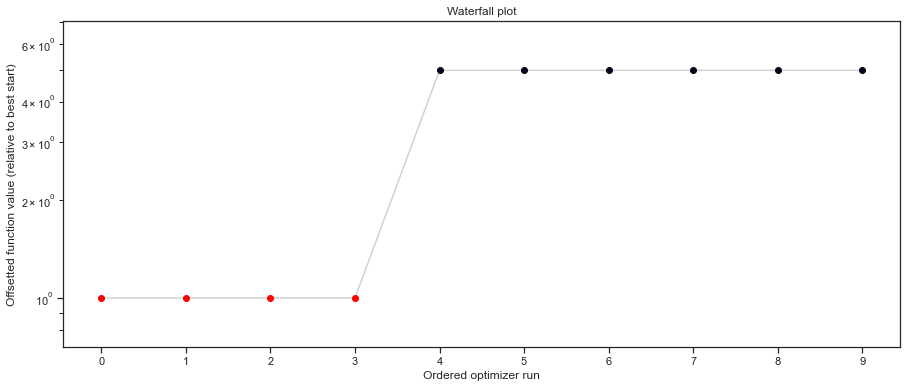
# plot waterfalls
pypesto.visualize.waterfall(result, size=(15,6))
[27]:
<AxesSubplot:title={'center':'Waterfall plot'}, xlabel='Ordered optimizer run', ylabel='Offsetted function value (relative to best start)'>
[28]:
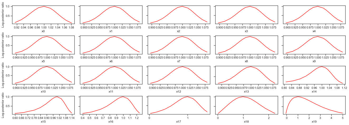
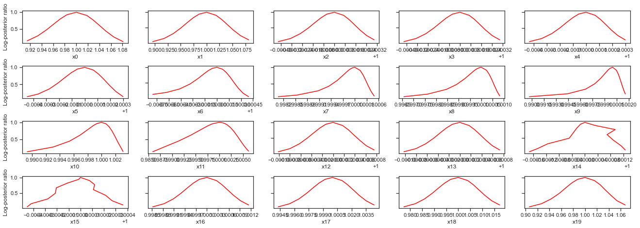
# plot profiles
pypesto.visualize.profiles(result)
[28]:
[<AxesSubplot:xlabel='x0', ylabel='Log-posterior ratio'>,
 <AxesSubplot:xlabel='x1'>,
 <AxesSubplot:xlabel='x2'>,
 <AxesSubplot:xlabel='x3'>,
 <AxesSubplot:xlabel='x4'>,
 <AxesSubplot:xlabel='x5', ylabel='Log-posterior ratio'>,
 <AxesSubplot:xlabel='x6'>,
 <AxesSubplot:xlabel='x7'>,
 <AxesSubplot:xlabel='x8'>,
 <AxesSubplot:xlabel='x9'>,
 <AxesSubplot:xlabel='x10', ylabel='Log-posterior ratio'>,
 <AxesSubplot:xlabel='x11'>,
 <AxesSubplot:xlabel='x12'>,
 <AxesSubplot:xlabel='x13'>,
 <AxesSubplot:xlabel='x14'>,
 <AxesSubplot:xlabel='x15', ylabel='Log-posterior ratio'>,
 <AxesSubplot:xlabel='x16'>,
 <AxesSubplot:xlabel='x17'>,
 <AxesSubplot:xlabel='x18'>,
 <AxesSubplot:xlabel='x19'>]
[29]:
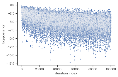
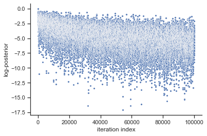
# plot samples
pypesto.visualize.sampling_fval_traces(result)
[29]:
<AxesSubplot:xlabel='iteration index', ylabel='log-posterior'>
Save result object in HDF5 File
[30]:
# create temporary file
fn = tempfile.mktemp(".hdf5")

# write result with write_result function.
# Choose which parts of the result object to save with
# corresponding booleans.
store.write_result(result=result,
                   filename=fn,
                   problem=True,
                   optimize=True,
                   profile=True,
                   sample=True)
Reload results
[31]:
# Read result
result2 = store.read_result(fn)
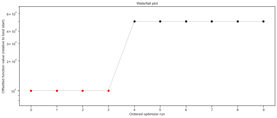
Plot (reloaded) results
[32]:
# plot waterfalls
pypesto.visualize.waterfall(result2, size=(15,6))
[32]:
<AxesSubplot:title={'center':'Waterfall plot'}, xlabel='Ordered optimizer run', ylabel='Offsetted function value (relative to best start)'>
[33]:
# plot profiles
pypesto.visualize.profiles(result2)
[33]:
[<AxesSubplot:xlabel='x0', ylabel='Log-posterior ratio'>,
 <AxesSubplot:xlabel='x1'>,
 <AxesSubplot:xlabel='x2'>,
 <AxesSubplot:xlabel='x3'>,
 <AxesSubplot:xlabel='x4'>,
 <AxesSubplot:xlabel='x5', ylabel='Log-posterior ratio'>,
 <AxesSubplot:xlabel='x6'>,
 <AxesSubplot:xlabel='x7'>,
 <AxesSubplot:xlabel='x8'>,
 <AxesSubplot:xlabel='x9'>,
 <AxesSubplot:xlabel='x10', ylabel='Log-posterior ratio'>,
 <AxesSubplot:xlabel='x11'>,
 <AxesSubplot:xlabel='x12'>,
 <AxesSubplot:xlabel='x13'>,
 <AxesSubplot:xlabel='x14'>,
 <AxesSubplot:xlabel='x15', ylabel='Log-posterior ratio'>,
 <AxesSubplot:xlabel='x16'>,
 <AxesSubplot:xlabel='x17'>,
 <AxesSubplot:xlabel='x18'>,
 <AxesSubplot:xlabel='x19'>]
[34]:
# plot samples
pypesto.visualize.sampling_fval_traces(result2)
[34]:
<AxesSubplot:xlabel='iteration index', ylabel='log-posterior'>
For the saving of optimization history, we refer to store.ipynb.