Rosenbrock banana
Here, we perform optimization for the Rosenbrock banana function, which does not require an AMICI model. In particular, we try several ways of specifying derivative information.
[1]:
import pypesto
import pypesto.visualize as visualize
import numpy as np
import scipy as sp
import matplotlib.pyplot as plt
from mpl_toolkits.mplot3d import Axes3D

%matplotlib inline
Define the objective and problem
[2]:
# first type of objective
objective1 = pypesto.Objective(fun=sp.optimize.rosen,
                               grad=sp.optimize.rosen_der,
                               hess=sp.optimize.rosen_hess)

# second type of objective
def rosen2(x):
    return (sp.optimize.rosen(x),
            sp.optimize.rosen_der(x),
            sp.optimize.rosen_hess(x))
objective2 = pypesto.Objective(fun=rosen2, grad=True, hess=True)

dim_full = 10
lb = -5 * np.ones((dim_full, 1))
ub = 5 * np.ones((dim_full, 1))

problem1 = pypesto.Problem(objective=objective1, lb=lb, ub=ub)
problem2 = pypesto.Problem(objective=objective2, lb=lb, ub=ub)
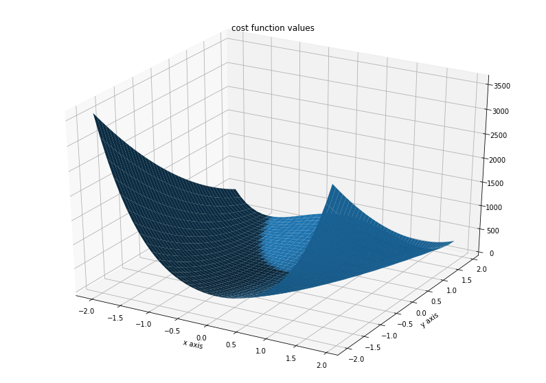
Illustration
[3]:
x = np.arange(-2, 2, 0.1)
y = np.arange(-2, 2, 0.1)
x, y = np.meshgrid(x, y)
z = np.zeros_like(x)
for j in range(0, x.shape[0]):
    for k in range(0, x.shape[1]):
        z[j,k] = objective1([x[j,k], y[j,k]], (0,))
[4]:
fig = plt.figure()
fig.set_size_inches(*(14,10))
ax = plt.axes(projection='3d')
ax.plot_surface(X=x, Y=y, Z=z)
plt.xlabel('x axis')
plt.ylabel('y axis')
ax.set_title('cost function values')
[4]:
Text(0.5, 0.92, 'cost function values')
Run optimization
[5]:
import pypesto.optimize as optimize
[6]:
%%time

# create different optimizers
optimizer_bfgs = optimize.ScipyOptimizer(method='l-bfgs-b')
optimizer_tnc = optimize.ScipyOptimizer(method='TNC')
optimizer_dogleg = optimize.ScipyOptimizer(method='dogleg')

# set number of starts
n_starts = 20

# save optimizer trace
history_options = pypesto.HistoryOptions(trace_record=True)

# Run optimizaitons for different optimzers
result1_bfgs = optimize.minimize(
    problem=problem1, optimizer=optimizer_bfgs,
    n_starts=n_starts, history_options=history_options)
result1_tnc = optimize.minimize(
    problem=problem1, optimizer=optimizer_tnc,
    n_starts=n_starts, history_options=history_options)
result1_dogleg = optimize.minimize(
    problem=problem1, optimizer=optimizer_dogleg,
    n_starts=n_starts, history_options=history_options)

# Optimize second type of objective
result2 = optimize.minimize(
    problem=problem2, optimizer=optimizer_tnc, n_starts=n_starts)
Function values from history and optimizer do not match: 2.685929315976887, 2.9820162443657527
Parameters obtained from history and optimizer do not match: [ 9.81668828e-01  9.70664899e-01  9.44081691e-01  8.86185728e-01
  7.98866760e-01  6.27503392e-01  3.49193984e-01  1.00863999e-01
  1.18119992e-02 -4.83096174e-04], [0.98232811 0.9607169  0.93006041 0.86376905 0.72679074 0.51464422
 0.25715153 0.03390018 0.0134388  0.00224348]
Function values from history and optimizer do not match: 2.932320470464073, 3.104833804292291
Parameters obtained from history and optimizer do not match: [9.85695690e-01 9.66998320e-01 9.34405532e-01 8.72211105e-01
 7.61716907e-01 5.82160864e-01 2.90132686e-01 5.88015713e-02
 1.02493152e-02 1.44786818e-04], [9.76820249e-01 9.49203293e-01 9.03611145e-01 8.32711736e-01
 6.92021069e-01 4.71244784e-01 2.26981271e-01 1.93600745e-02
 9.06285841e-03 3.00716108e-04]
Function values from history and optimizer do not match: 7.128857018893593, 7.737539574292646
Parameters obtained from history and optimizer do not match: [-9.74521002e-01  9.48916364e-01  8.98382180e-01  7.95485807e-01
  6.32334509e-01  3.95389632e-01  1.55262583e-01  2.24615758e-02
  9.92812211e-03  4.70538835e-05], [-0.95137113  0.92287756  0.85600385  0.74220324  0.53469862  0.25223695
  0.05388462  0.01175751  0.01035533  0.00121333]
Function values from history and optimizer do not match: 4.047666500407507, 4.8092850089870245
Parameters obtained from history and optimizer do not match: [9.57097378e-01 9.15272882e-01 8.35583627e-01 6.92924153e-01
 4.69156347e-01 1.98916115e-01 2.87951418e-02 1.21495892e-02
 1.14276335e-02 2.48487865e-04], [9.37837181e-01 8.73541886e-01 7.61292462e-01 5.64720865e-01
 2.84119482e-01 6.17767487e-02 1.53662912e-02 1.54992154e-02
 1.49513982e-02 2.98560604e-04]
Function values from history and optimizer do not match: 4.760963749486806, 5.255690010134404
Parameters obtained from history and optimizer do not match: [-0.98990379  0.98886801  0.98189121  0.96587616  0.93451723  0.87262109
  0.75889559  0.56883791  0.31364781  0.07883034], [-0.99248035  0.99162316  0.97889433  0.95364865  0.91078502  0.8261375
  0.68236478  0.45820395  0.17444197  0.01383626]
Function values from history and optimizer do not match: 1.8159939922237558, 2.5425135960926237
Parameters obtained from history and optimizer do not match: [9.90583524e-01 9.80917081e-01 9.63072632e-01 9.30325108e-01
 8.61713989e-01 7.40678602e-01 5.38268550e-01 2.71328618e-01
 5.43996813e-02 7.89698144e-04], [9.89162276e-01 9.78043570e-01 9.51094059e-01 9.02211862e-01
 8.07645490e-01 6.35406055e-01 3.75384767e-01 1.11075371e-01
 1.30319964e-02 2.11963742e-04]
Function values from history and optimizer do not match: 2.2546577084566284, 2.988463828057193
Parameters obtained from history and optimizer do not match: [9.86890406e-01 9.73738159e-01 9.51089323e-01 9.02086672e-01
 8.09027663e-01 6.46629154e-01 4.04671023e-01 1.51442890e-01
 1.94187285e-02 2.45054194e-04], [9.81148194e-01 9.60640784e-01 9.21690034e-01 8.55030060e-01
 7.31180374e-01 5.23069013e-01 2.44624625e-01 3.39441804e-02
 1.03741576e-02 2.45306769e-05]
Function values from history and optimizer do not match: 0.3545683077008359, 0.5906121485206447
Parameters obtained from history and optimizer do not match: [0.99668472 0.99262575 0.98945665 0.98129911 0.96532923 0.93081497
 0.86315388 0.74328951 0.53910453 0.2736718 ], [0.9963228  0.99215562 0.98514259 0.97132273 0.94683482 0.89670025
 0.80300196 0.64224614 0.40061592 0.14210795]
Function values from history and optimizer do not match: 1.442951465698237, 2.117657844069939
Parameters obtained from history and optimizer do not match: [0.99253701 0.98698288 0.97438388 0.94864025 0.89249411 0.79343394
 0.62110958 0.37154848 0.12142293 0.00337751], [9.85576055e-01 9.72515609e-01 9.52500598e-01 9.14984751e-01
 8.40282960e-01 7.07108893e-01 4.93844010e-01 2.19299261e-01
 1.80684261e-02 2.39353088e-04]
Function values from history and optimizer do not match: 0.4310215367360306, 0.7200757805862191
Parameters obtained from history and optimizer do not match: [0.99728801 0.99265292 0.98655945 0.97724776 0.95330363 0.91375386
 0.83290125 0.68949822 0.4687524  0.21461214], [0.99666432 0.99530499 0.9871224  0.96976884 0.94230384 0.89383977
 0.79420195 0.62752848 0.3793222  0.11129682]
Function values from history and optimizer do not match: 6.33997905147026, 7.069668392692864
Parameters obtained from history and optimizer do not match: [7.84450616e-01 6.10188497e-01 3.64032562e-01 1.19476022e-01
 1.25200919e-02 9.74166479e-03 1.00503247e-02 8.51949533e-03
 9.92120699e-03 1.97235559e-04], [ 7.13358486e-01  4.93846146e-01  2.05601150e-01  2.46828697e-02
  1.00531820e-02  8.83759494e-03  9.93584452e-03  1.16356575e-02
  1.00772170e-02 -9.19777874e-05]
Function values from history and optimizer do not match: 1.080010188007246, 1.638996874292531
Parameters obtained from history and optimizer do not match: [0.99354151 0.98796198 0.97743947 0.96147507 0.92290179 0.84825176
 0.71159467 0.49318554 0.223647   0.03035961], [0.99093761 0.98310117 0.96952353 0.94165684 0.88399848 0.77718421
 0.59296742 0.3287277  0.08605952 0.00216266]
Function values from history and optimizer do not match: 6.334069745693479, 7.027921368861192
Parameters obtained from history and optimizer do not match: [-0.98264119  0.97390376  0.94694027  0.8905699   0.79188661  0.62198099
  0.37540054  0.12148722  0.01380672  0.00504649], [-0.97385408  0.95844934  0.9257917   0.85697013  0.71970238  0.49533252
  0.21270446  0.03011495  0.00979574 -0.00651404]
CPU times: user 2.74 s, sys: 37.7 ms, total: 2.78 s
Wall time: 2.74 s
Visualize and compare optimization results
[7]:
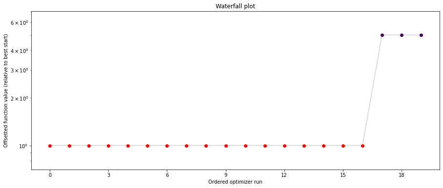
# plot separated waterfalls
visualize.waterfall(result1_bfgs, size=(15,6))
visualize.waterfall(result1_tnc, size=(15,6))
visualize.waterfall(result1_dogleg, size=(15,6))
[7]:
<matplotlib.axes._subplots.AxesSubplot at 0x7fb3be1ba0d0>
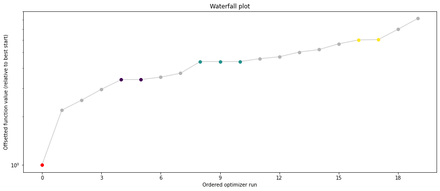
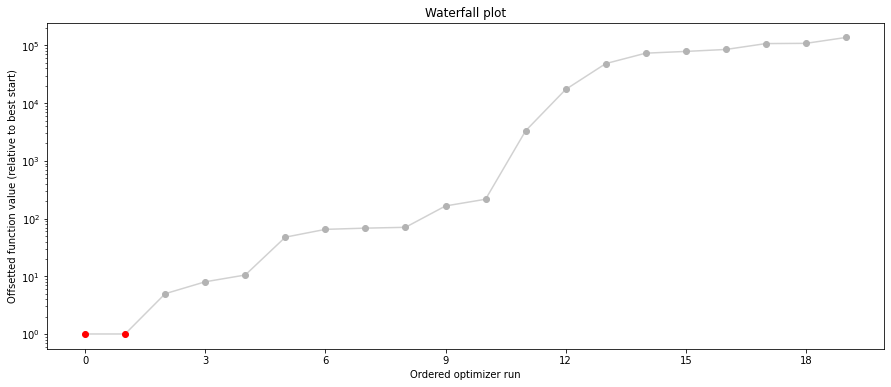
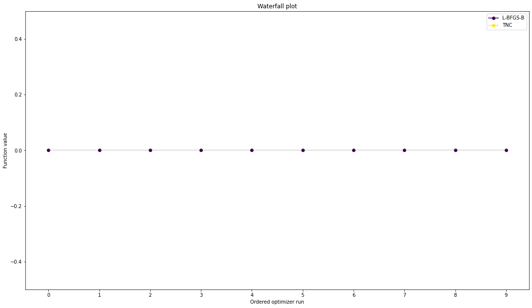
We can now have a closer look, which method perfomred better: Let’s first compare bfgs and TNC, since both methods gave good results. How does the fine convergence look like?
[8]:
# plot one list of waterfalls
visualize.waterfall([result1_bfgs, result1_tnc],
                    legends=['L-BFGS-B', 'TNC'],
                    start_indices=10,
                    scale_y='lin')
[8]:
<matplotlib.axes._subplots.AxesSubplot at 0x7fb3bf463760>
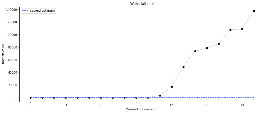
[9]:
# retrieve second optimum
all_x = result1_bfgs.optimize_result.get_for_key('x')
all_fval = result1_bfgs.optimize_result.get_for_key('fval')
x = all_x[19]
fval = all_fval[19]
print('Second optimum at: ' + str(fval))

# create a reference point from it
ref = {'x': x, 'fval': fval, 'color': [
    0.2, 0.4, 1., 1.], 'legend': 'second optimum'}
ref = visualize.create_references(ref)

# new waterfall plot with reference point for second optimum
visualize.waterfall(result1_dogleg, size=(15,6),
                    scale_y='lin', y_limits=[-1, 101],
                    reference=ref, colors=[0., 0., 0., 1.])
Second optimum at: 3.9865791142048876
[9]:
<matplotlib.axes._subplots.AxesSubplot at 0x7fb3bde83940>
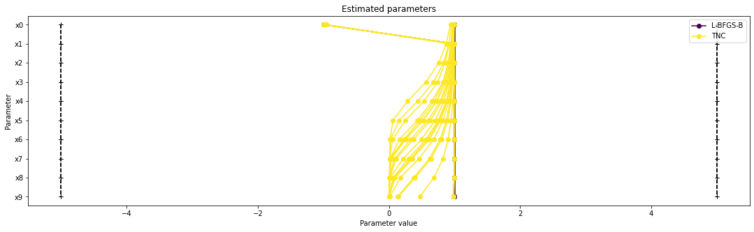
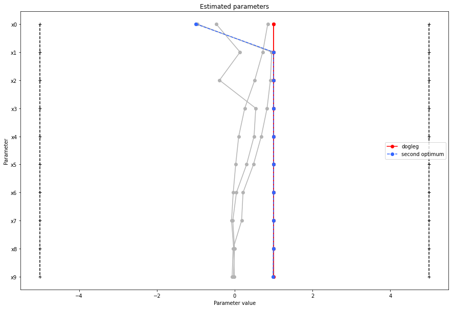
Visualize parameters
There seems to be a second local optimum. We want to see whether it was also found by the dogleg method
[10]:
visualize.parameters([result1_bfgs, result1_tnc],
                     legends=['L-BFGS-B', 'TNC'],
                     balance_alpha=False)
visualize.parameters(result1_dogleg,
                     legends='dogleg',
                     reference=ref,
                     size=(15,10),
                     start_indices=[0, 1, 2, 3, 4, 5],
                     balance_alpha=False)
[10]:
<matplotlib.axes._subplots.AxesSubplot at 0x7fb3bdd5b430>
If the result needs to be examined in more detail, it can easily be exported as a pandas.DataFrame:
[11]:
df = result1_tnc.optimize_result.as_dataframe(
    ['fval', 'n_fval', 'n_grad', 'n_hess', 'n_res', 'n_sres', 'time'])
df.head()
[11]:
| fval | n_fval | n_grad | n_hess | n_res | n_sres | time | |
|---|---|---|---|---|---|---|---|
| 0 | 0.590612 | 101 | 101 | 0 | 0 | 0 | 0.052775 |
| 1 | 1.779748 | 101 | 101 | 0 | 0 | 0 | 0.049476 |
| 2 | 2.117658 | 101 | 101 | 0 | 0 | 0 | 0.039615 |
| 3 | 2.542514 | 101 | 101 | 0 | 0 | 0 | 0.064188 |
| 4 | 2.982016 | 101 | 101 | 0 | 0 | 0 | 0.024157 |
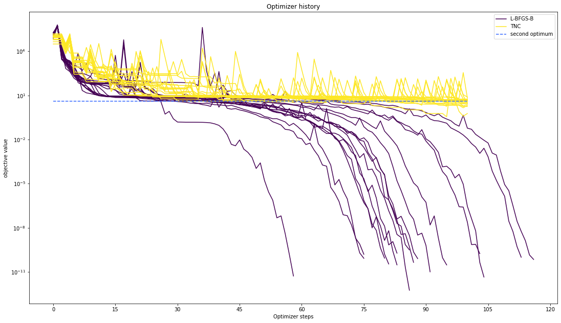
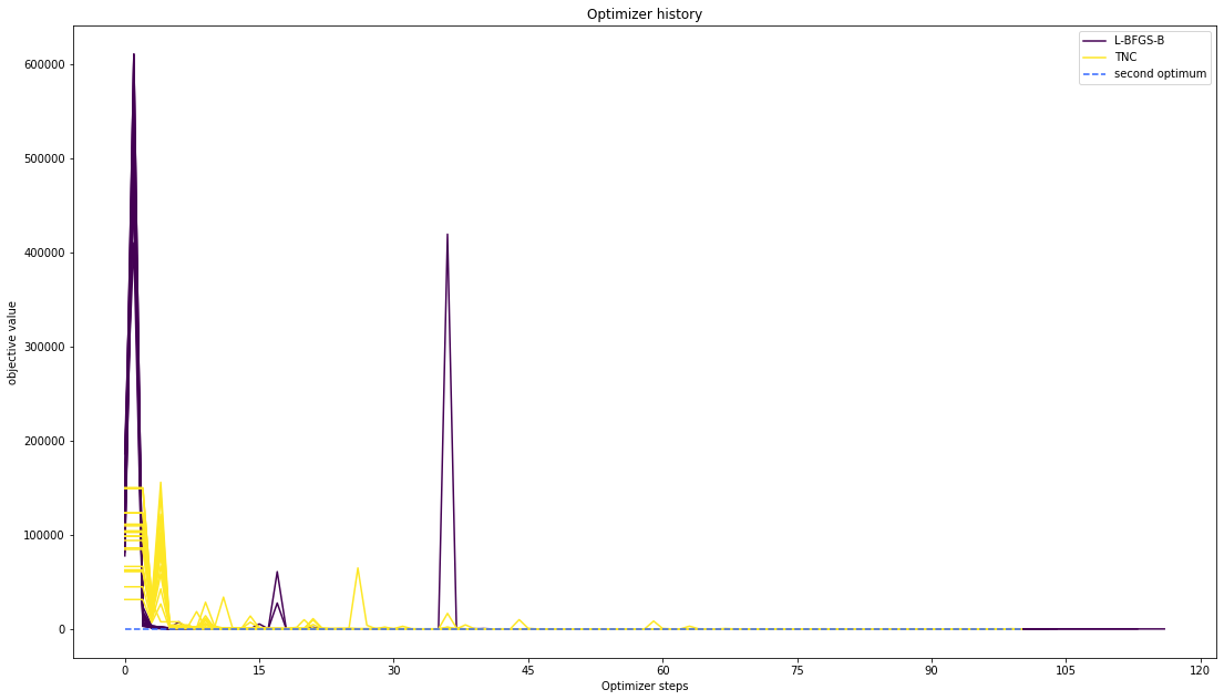
Optimizer history
Let’s compare optimzer progress over time.
[12]:
# plot one list of waterfalls
visualize.optimizer_history([result1_bfgs, result1_tnc],
                            legends=['L-BFGS-B', 'TNC'],
                            reference=ref)
# plot one list of waterfalls
visualize.optimizer_history(result1_dogleg,
                            reference=ref)
[12]:
<matplotlib.axes._subplots.AxesSubplot at 0x7fb3bdbcc820>
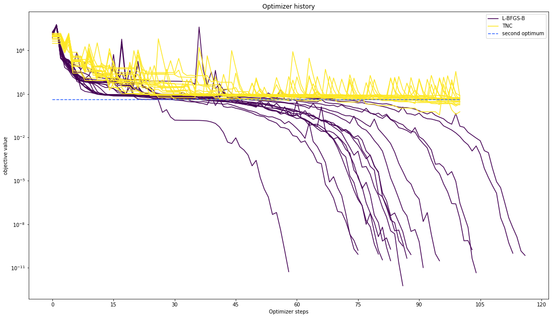
We can also visualize this usign other scalings or offsets…
[13]:
# plot one list of waterfalls
visualize.optimizer_history([result1_bfgs, result1_tnc],
                            legends=['L-BFGS-B', 'TNC'],
                            reference=ref,
                            offset_y=0.)

# plot one list of waterfalls
visualize.optimizer_history([result1_bfgs, result1_tnc],
                            legends=['L-BFGS-B', 'TNC'],
                            reference=ref,
                            scale_y='lin',
                            y_limits=[-1., 11.])
[13]:
<matplotlib.axes._subplots.AxesSubplot at 0x7fb3be01d130>
Compute profiles
The profiling routine needs a problem, a results object and an optimizer.
Moreover it accepts an index of integer (profile_index), whether or not a profile should be computed.
Finally, an integer (result_index) can be passed, in order to specify the local optimum, from which profiling should be started.
[14]:
import pypesto.profile as profile
[15]:
%%time

# compute profiles
profile_options = profile.ProfileOptions(min_step_size=0.0005,
    delta_ratio_max=0.05,
    default_step_size=0.005,
    ratio_min=0.01)

result1_bfgs = profile.parameter_profile(
    problem=problem1,
    result=result1_bfgs,
    optimizer=optimizer_bfgs,
    profile_index=np.array([1, 1, 1, 0, 0, 1, 0, 1, 0, 0, 0]),
    result_index=0,
    profile_options=profile_options)

# compute profiles from second optimum
result1_bfgs = profile.parameter_profile(
    problem=problem1,
    result=result1_bfgs,
    optimizer=optimizer_bfgs,
    profile_index=np.array([1, 1, 1, 0, 0, 1, 0, 1, 0, 0, 0]),
    result_index=19,
    profile_options=profile_options)
CPU times: user 1.31 s, sys: 4.28 ms, total: 1.32 s
Wall time: 1.32 s
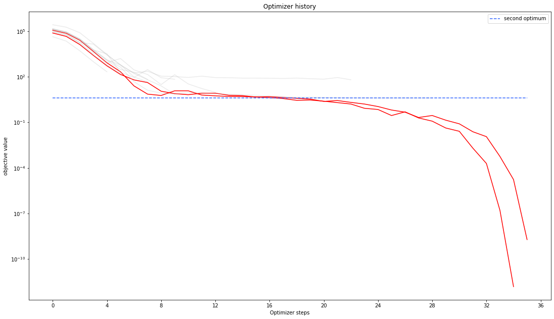
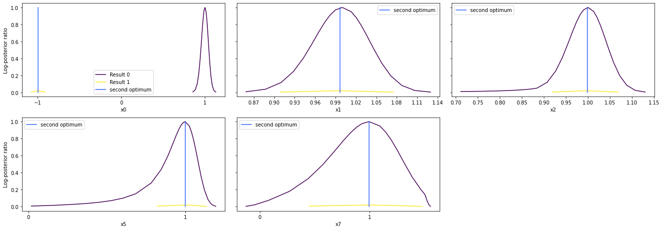
Visualize and analyze results
pypesto offers easy-to-use visualization routines:
[16]:
# specify the parameters, for which profiles should be computed
ax = visualize.profiles(result1_bfgs, profile_indices = [0,1,2,5,7],
                        reference=ref, profile_list_ids=[0, 1])
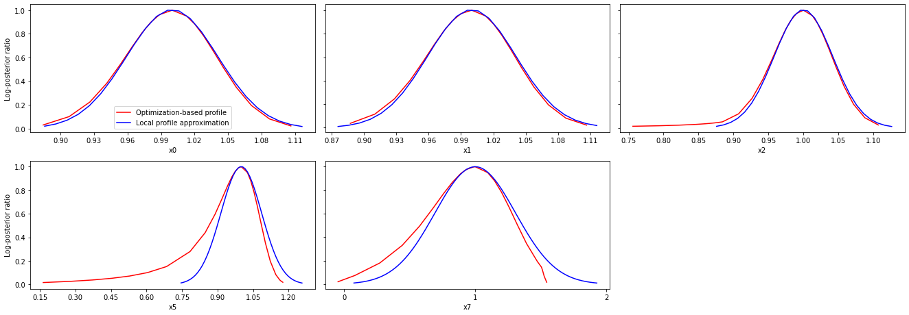
Approximate profiles
When computing the profiles is computationally too demanding, it is possible to employ to at least consider a normal approximation with covariance matrix given by the Hessian or FIM at the optimal parameters.
[17]:
%%time

result1_tnc = profile.approximate_parameter_profile(
    problem=problem1,
    result=result1_bfgs,
    profile_index=np.array([1, 1, 1, 0, 0, 1, 0, 1, 0, 0, 0]),
    result_index=0,
    n_steps=1000)
CPU times: user 25 ms, sys: 16.3 ms, total: 41.4 ms
Wall time: 24.2 ms
These approximate profiles require at most one additional function evaluation, can however yield substantial approximation errors:
[18]:
axes = visualize.profiles(
    result1_bfgs, profile_indices = [0,1,2,5,7], profile_list_ids=[0, 2],
    ratio_min=0.01, colors=[(1,0,0,1), (0,0,1,1)],
    legends=["Optimization-based profile", "Local profile approximation"])
We can also plot approximate confidence intervals based on profiles:
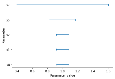
[19]:
visualize.profile_cis(
    result1_bfgs, confidence_level=0.95, profile_list=2)
[19]:
<matplotlib.axes._subplots.AxesSubplot at 0x7fb3bda13f10>