Rosenbrock banana

Here, we perform optimization for the Rosenbrock banana function, which does not require an AMICI model. In particular, we try several ways of specifying derivative information.

import pypesto
import numpy as np
import scipy as sp
import matplotlib.pyplot as plt
from mpl_toolkits.mplot3d import Axes3D

%matplotlib inline

Define the objective and problem

# first type of objective
objective1 = pypesto.Objective(fun=sp.optimize.rosen,
                               grad=sp.optimize.rosen_der,
                               hess=sp.optimize.rosen_hess)

# second type of objective
def rosen2(x):
    return sp.optimize.rosen(x), sp.optimize.rosen_der(x), sp.optimize.rosen_hess(x)
objective2 = pypesto.Objective(fun=rosen2, grad=True, hess=True)

dim_full = 10
lb = -2 * np.ones((dim_full, 1))
ub = 2 * np.ones((dim_full, 1))

problem1 = pypesto.Problem(objective=objective1, lb=lb, ub=ub)
problem2 = pypesto.Problem(objective=objective2, lb=lb, ub=ub)

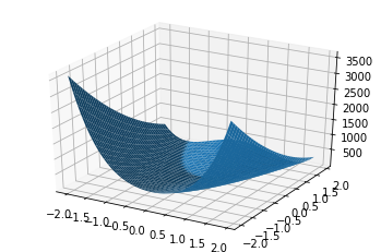
Illustration

x = np.arange(-2, 2, 0.1)
y = np.arange(-2, 2, 0.1)
x, y = np.meshgrid(x, y)
z = np.zeros_like(x)
for j in range(0, x.shape[0]):
    for k in range(0, x.shape[1]):
        z[j,k] = objective1([x[j,k], y[j,k]], (0,))

fig = plt.figure()
ax = plt.axes(projection='3d')
ax.plot_surface(X=x, Y=y, Z=z)

<mpl_toolkits.mplot3d.art3d.Poly3DCollection at 0x121e42908>

Run optimization

optimizer = pypesto.ScipyOptimizer()
n_starts = 20

result1 = pypesto.minimize(problem=problem1, optimizer=optimizer, n_starts=n_starts)
result2 = pypesto.minimize(problem=problem2, optimizer=optimizer, n_starts=n_starts)

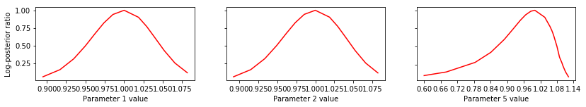
Compute profiles

The profiling routine needs a problem, a results object and an optimizer.

Moreover it accepts an index of integer (profile_index), whether or not a profile should be computed.

Finally, an integer (result_index) can be passed, in order to specify the local optimum, from which profiling should be started.

result1 = pypesto.parameter_profile(
    problem=problem1,
    result=result1,
    optimizer=optimizer,
    profile_index=np.array([0, 1, 1, 0, 0, 1, 0, 1, 0, 0, 0]),
    result_index=1)

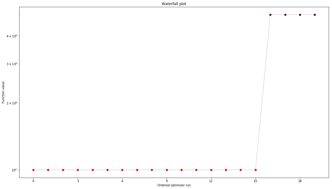
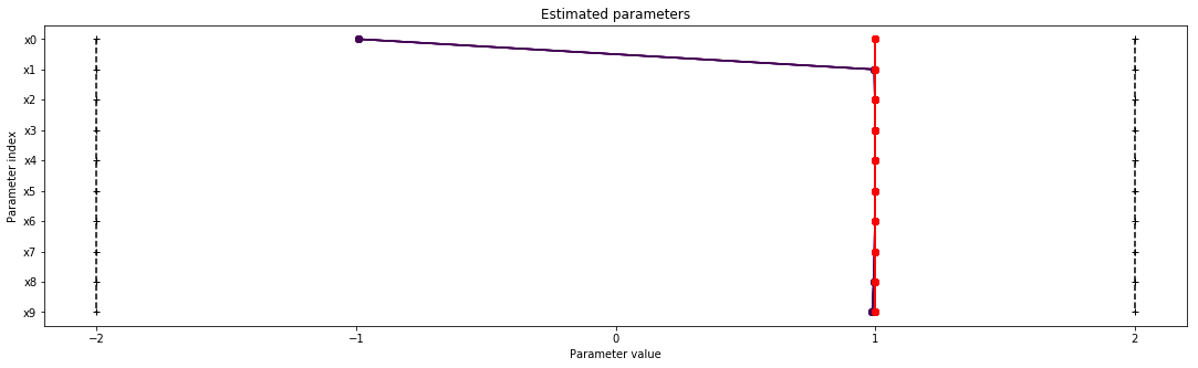
Visualize and analyze results

pypesto offers easy-to-use visualization routines:

import pypesto.visualize

pypesto.visualize.waterfall(result1)
pypesto.visualize.parameters(result1)

# specify the parameters, for which profiles should be computed
pypesto.visualize.profiles(result1, profile_indices = [1,2,5])

[<matplotlib.axes._subplots.AxesSubplot at 0x124363d68>,
 <matplotlib.axes._subplots.AxesSubplot at 0x1245114a8>,
 <matplotlib.axes._subplots.AxesSubplot at 0x1245230f0>]

If the result needs to be examined in more detail, it can easily be exported as a pandas.DataFrame:

result1.optimize_result.as_dataframe(['fval', 'n_fval', 'n_grad', 'n_hess', 'n_res', 'n_sres', 'time'])

	fval	n_fval	n_grad	n_hess	n_res	n_sres	time
0	3.864669e-12	89	89	0	0	0	0.016705
1	5.391376e-12	83	83	0	0	0	0.015477
2	6.878944e-12	88	88	0	0	0	0.119707
3	7.215911e-12	91	91	0	0	0	0.037070
4	9.545020e-12	69	69	0	0	0	0.022376
5	1.244748e-11	83	83	0	0	0	0.022337
6	1.263889e-11	88	88	0	0	0	0.018748
7	1.562623e-11	86	86	0	0	0	0.022854
8	4.085166e-11	73	73	0	0	0	0.011622
9	7.246517e-11	79	79	0	0	0	0.026188
10	8.612691e-11	67	67	0	0	0	0.012368
11	1.823874e-10	76	76	0	0	0	0.013582
12	1.861598e-10	78	78	0	0	0	0.046079
13	1.922645e-10	90	90	0	0	0	0.025491
14	2.231378e-10	89	89	0	0	0	0.021747
15	2.499322e-10	73	73	0	0	0	0.042578
16	3.054340e-10	81	81	0	0	0	0.018495
17	3.370285e-10	76	76	0	0	0	0.017206
18	1.678268e-09	75	75	0	0	0	0.014224
19	3.986579e+00	71	71	0	0	0	0.043969