Rosenbrock banana
Here, we perform optimization for the Rosenbrock banana function, which does not require an AMICI model. In particular, we try several ways of specifying derivative information.
[1]:
import pypesto
import numpy as np
import scipy as sp
import matplotlib.pyplot as plt
from mpl_toolkits.mplot3d import Axes3D

%matplotlib inline
Define the objective and problem
[2]:
# first type of objective
objective1 = pypesto.Objective(fun=sp.optimize.rosen,
                               grad=sp.optimize.rosen_der,
                               hess=sp.optimize.rosen_hess)

# second type of objective
def rosen2(x):
    return sp.optimize.rosen(x), sp.optimize.rosen_der(x), sp.optimize.rosen_hess(x)
objective2 = pypesto.Objective(fun=rosen2, grad=True, hess=True)

dim_full = 10
lb = -5 * np.ones((dim_full, 1))
ub = 5 * np.ones((dim_full, 1))

problem1 = pypesto.Problem(objective=objective1, lb=lb, ub=ub)
problem2 = pypesto.Problem(objective=objective2, lb=lb, ub=ub)
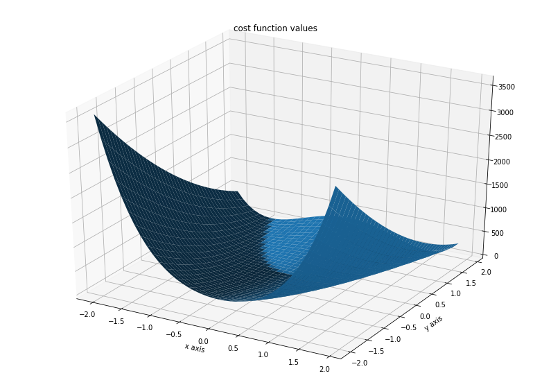
Illustration
[3]:
x = np.arange(-2, 2, 0.1)
y = np.arange(-2, 2, 0.1)
x, y = np.meshgrid(x, y)
z = np.zeros_like(x)
for j in range(0, x.shape[0]):
    for k in range(0, x.shape[1]):
        z[j,k] = objective1([x[j,k], y[j,k]], (0,))
[4]:
fig = plt.figure()
fig.set_size_inches(*(14,10))
ax = plt.axes(projection='3d')
ax.plot_surface(X=x, Y=y, Z=z)
plt.xlabel('x axis')
plt.ylabel('y axis')
ax.set_title('cost function values')
[4]:
Text(0.5, 0.92, 'cost function values')
Run optimization
[5]:
# create different optimizers
optimizer_bfgs = pypesto.ScipyOptimizer(method='l-bfgs-b')
optimizer_tnc = pypesto.ScipyOptimizer(method='TNC')
optimizer_dogleg = pypesto.ScipyOptimizer(method='dogleg')

# set number of starts
n_starts = 20

# save optimizer trace
history_options = pypesto.HistoryOptions(trace_record=True)

# Run optimizaitons for different optimzers
result1_bfgs = pypesto.minimize(
    problem=problem1, optimizer=optimizer_bfgs,
    n_starts=n_starts, history_options=history_options)
result1_tnc = pypesto.minimize(
    problem=problem1, optimizer=optimizer_tnc,
    n_starts=n_starts, history_options=history_options)
result1_dogleg = pypesto.minimize(
    problem=problem1, optimizer=optimizer_dogleg,
    n_starts=n_starts, history_options=history_options)

# Optimize second type of objective
result2 = pypesto.minimize(problem=problem2, optimizer=optimizer_tnc, n_starts=n_starts)
Visualize and compare optimization results
[6]:
import pypesto.visualize
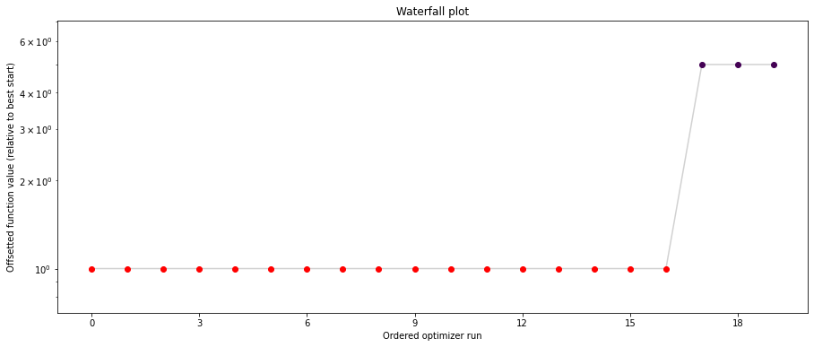
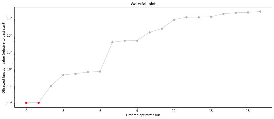
# plot separated waterfalls
pypesto.visualize.waterfall(result1_bfgs, size=(15,6))
pypesto.visualize.waterfall(result1_tnc, size=(15,6))
pypesto.visualize.waterfall(result1_dogleg, size=(15,6))
[6]:
<matplotlib.axes._subplots.AxesSubplot at 0x7fd9397beb90>

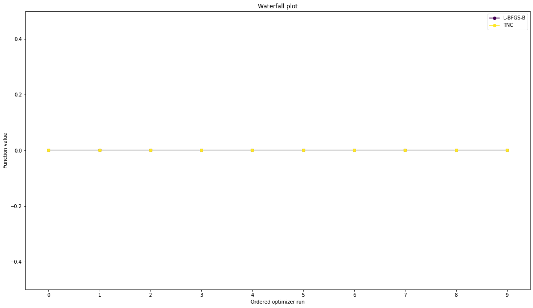
We can now have a closer look, which method perfomred better: Let’s first compare bfgs and TNC, since both methods gave good results. How does the fine convergence look like?
[7]:
# plot one list of waterfalls
pypesto.visualize.waterfall([result1_bfgs, result1_tnc],
                            legends=['L-BFGS-B', 'TNC'],
                            start_indices=10,
                            scale_y='lin')
[7]:
<matplotlib.axes._subplots.AxesSubplot at 0x7fd93936a410>
[8]:
# retrieve second optimum
all_x = result1_bfgs.optimize_result.get_for_key('x')
all_fval = result1_bfgs.optimize_result.get_for_key('fval')
x = all_x[19]
fval = all_fval[19]
print('Second optimum at: ' + str(fval))
# create a reference point from it
ref = {'x': x, 'fval': fval, 'color': [
0.2, 0.4, 1., 1.], 'legend': 'second optimum'}
ref = pypesto.visualize.create_references(ref)
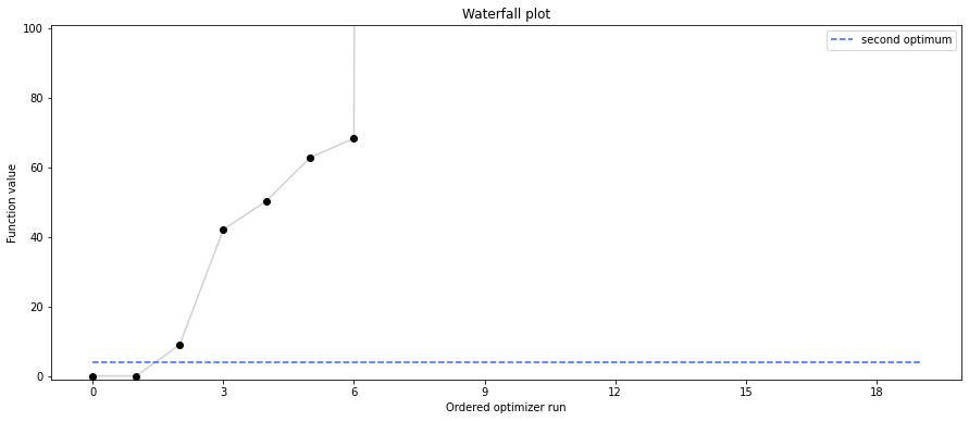
# new waterfall plot with reference point for second optimum
pypesto.visualize.waterfall(result1_dogleg, size=(15,6),
scale_y='lin', y_limits=[-1, 101],
reference=ref, colors=[0., 0., 0., 1.])
Second optimum at: 3.9865791124344874
[8]:
<matplotlib.axes._subplots.AxesSubplot at 0x7fd9393120d0>
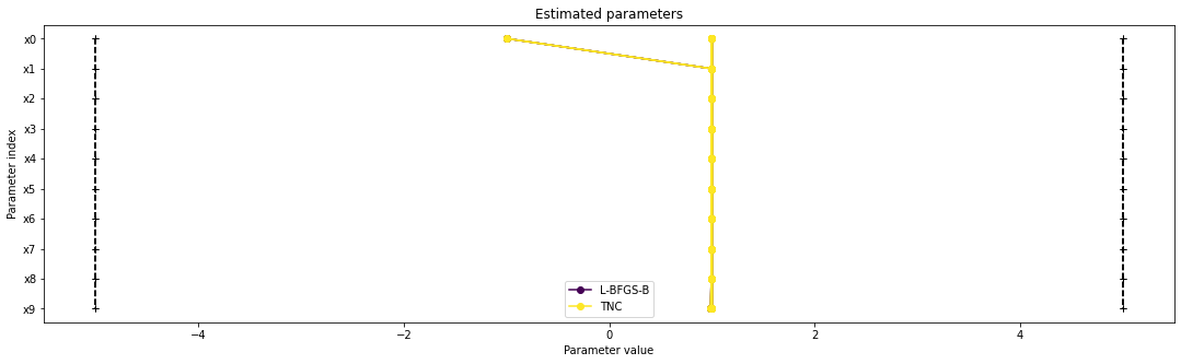
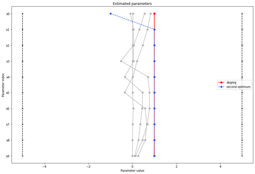
Visualize parameters
There seems to be a second local optimum. We want to see whether it was also found by the dogleg method
[9]:
pypesto.visualize.parameters([result1_bfgs, result1_tnc],
                            legends=['L-BFGS-B', 'TNC'],
                            balance_alpha=False)
pypesto.visualize.parameters(result1_dogleg,
                             legends='dogleg',
                             reference=ref,
                             size=(15,10),
                             start_indices=[0, 1, 2, 3, 4, 5],
                             balance_alpha=False)
[9]:
<matplotlib.axes._subplots.AxesSubplot at 0x7fd9394ccf10>
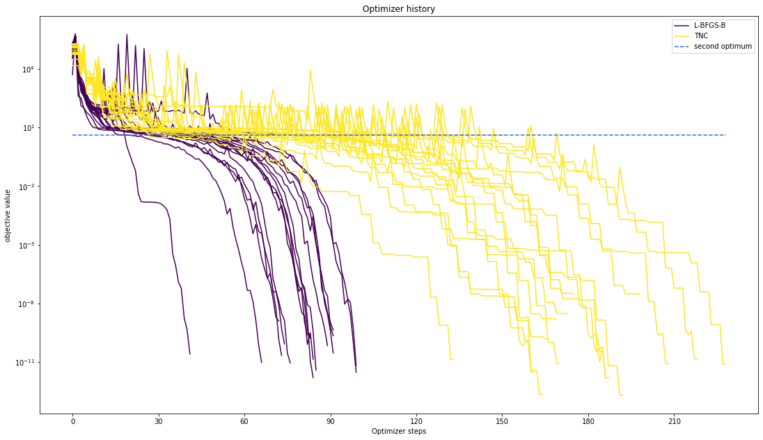
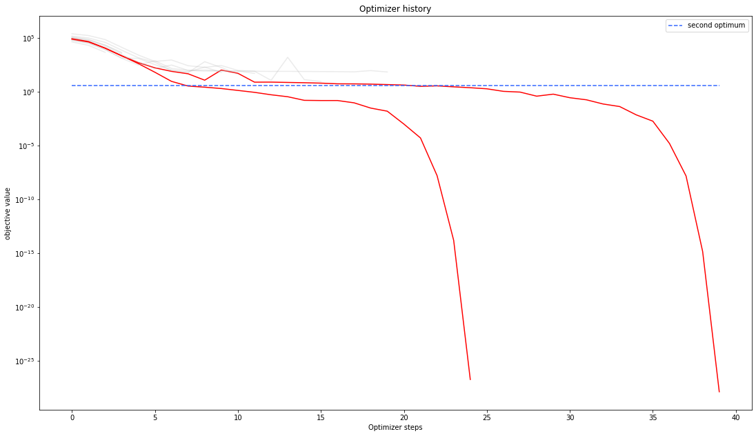
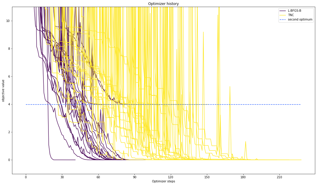
Optimizer history
Let’s compare optimzer progress over time.
[10]:
# plot one list of waterfalls
pypesto.visualize.optimizer_history([result1_bfgs, result1_tnc],
                                    legends=['L-BFGS-B', 'TNC'],
                                    reference=ref)
# plot one list of waterfalls
pypesto.visualize.optimizer_history(result1_dogleg,
                                    reference=ref)
[10]:
<matplotlib.axes._subplots.AxesSubplot at 0x7fd93983b750>
We can also visualize this usign other scalings or offsets…
[11]:
# plot one list of waterfalls
pypesto.visualize.optimizer_history([result1_bfgs, result1_tnc],
                                    legends=['L-BFGS-B', 'TNC'],
                                    reference=ref,
                                    offset_y=0.)

# plot one list of waterfalls
pypesto.visualize.optimizer_history([result1_bfgs, result1_tnc],
                                    legends=['L-BFGS-B', 'TNC'],
                                    reference=ref,
                                    scale_y='lin',
                                    y_limits=[-1., 11.])
[11]:
<matplotlib.axes._subplots.AxesSubplot at 0x7fd9390d9690>

Compute profiles
The profiling routine needs a problem, a results object and an optimizer.
Moreover it accepts an index of integer (profile_index), whether or not a profile should be computed.
Finally, an integer (result_index) can be passed, in order to specify the local optimum, from which profiling should be started.
[12]:
# compute profiles
profile_options = pypesto.ProfileOptions(min_step_size=0.0005,
    delta_ratio_max=0.05,
    default_step_size=0.005,
    ratio_min=0.03)

result1_tnc = pypesto.parameter_profile(
    problem=problem1,
    result=result1_tnc,
    optimizer=optimizer_tnc,
    profile_index=np.array([1, 1, 1, 0, 0, 1, 0, 1, 0, 0, 0]),
    result_index=0,
    profile_options=profile_options)

# compute profiles from second optimum
result1_tnc = pypesto.parameter_profile(
    problem=problem1,
    result=result1_tnc,
    optimizer=optimizer_tnc,
    profile_index=np.array([1, 1, 1, 0, 0, 1, 0, 1, 0, 0, 0]),
    result_index=19,
    profile_options=profile_options)
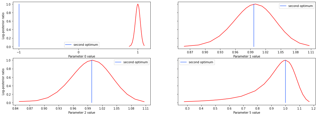
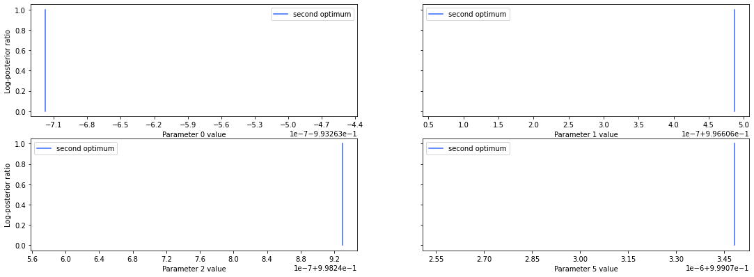
Visualize and analyze results
pypesto offers easy-to-use visualization routines:
[13]:
# specify the parameters, for which profiles should be computed
ax = pypesto.visualize.profiles(result1_tnc, profile_indices = [0,1,2,5],
                           reference=ref, profile_list_id=0)
# plot profiles again, now from second optimum
ax = pypesto.visualize.profiles(result1_tnc, profile_indices = [0,1,2,5],
                           reference=ref, profile_list_id=1)
If the result needs to be examined in more detail, it can easily be exported as a pandas.DataFrame:
[14]:
result1_tnc.optimize_result.as_dataframe(['fval', 'n_fval', 'n_grad',
                                          'n_hess', 'n_res', 'n_sres', 'time'])
[14]:
| fval | n_fval | n_grad | n_hess | n_res | n_sres | time | |
|---|---|---|---|---|---|---|---|
| 0 | 1.968227e-13 | 193 | 193 | 0 | 0 | 0 | 0.018201 |
| 1 | 2.202262e-13 | 165 | 165 | 0 | 0 | 0 | 0.039069 |
| 2 | 1.550811e-12 | 188 | 188 | 0 | 0 | 0 | 0.017980 |
| 3 | 1.553846e-12 | 188 | 188 | 0 | 0 | 0 | 0.017905 |
| 4 | 3.138476e-12 | 162 | 162 | 0 | 0 | 0 | 0.015469 |
| 5 | 8.042668e-12 | 229 | 229 | 0 | 0 | 0 | 0.021637 |
| 6 | 8.268731e-12 | 209 | 209 | 0 | 0 | 0 | 0.049976 |
| 7 | 8.310174e-12 | 171 | 171 | 0 | 0 | 0 | 0.016296 |
| 8 | 1.364149e-11 | 219 | 219 | 0 | 0 | 0 | 0.021103 |
| 9 | 1.382298e-11 | 134 | 134 | 0 | 0 | 0 | 0.013395 |
| 10 | 3.487863e-11 | 186 | 186 | 0 | 0 | 0 | 0.017843 |
| 11 | 1.211274e-10 | 160 | 160 | 0 | 0 | 0 | 0.042303 |
| 12 | 1.568336e-10 | 167 | 167 | 0 | 0 | 0 | 0.016380 |
| 13 | 1.557791e-09 | 170 | 170 | 0 | 0 | 0 | 0.016406 |
| 14 | 2.989273e-09 | 174 | 174 | 0 | 0 | 0 | 0.017172 |
| 15 | 3.045916e-08 | 199 | 199 | 0 | 0 | 0 | 0.026230 |
| 16 | 3.194012e-08 | 176 | 176 | 0 | 0 | 0 | 0.033760 |
| 17 | 3.986579e+00 | 134 | 134 | 0 | 0 | 0 | 0.013941 |
| 18 | 3.986579e+00 | 152 | 152 | 0 | 0 | 0 | 0.017177 |
| 19 | 3.986579e+00 | 103 | 103 | 0 | 0 | 0 | 0.009830 |